Supersymmetric Lagrangians

Supersymmetry has been discussed many times on this blog but a particular question on the Physics Stack Exchange today,

Why is the lightest Higgs not a free parameter in SUSY? (SE)

convinced me to write a new, not too long text about the way to construct minimally supersymmetric Lagrangians for \(d=4\) supersymmetric quantum field theories.

Just to be sure, the poster above asked why the Higgs mass seems to be freely adjustable in the Standard Model but there are various constraints on the Higgs mass in the Minimal Supersymmetric Standard Model – for example, the lighter Higgs mass can't be too much heavier than the Z-boson.

I answered that a heavy Higgs boson in the Standard Model also leads to some trouble such as instabilities but the bulk of my answer – which you can read if you click at the SE link above – was dedicated to an explanation why the Higgs masses can't be arbitrarily scaled in supersymmetric theories.



A short answer is that the quartic coupling \(\lambda\) in the \(\lambda h^4\) quartic (fourth-order) self-interaction of the Higgs field – which is an increasing function of the Higgs mass, assuming a fixed given vacuum expectation value (vev) – is no longer arbitrary in the MSSM. Instead, it is given by various combinations of \(g^2\) and \(g^{\prime 2}\) gauge couplings for the \(SU(2)\times U(1)\) electroweak gauge group. This follows from some insights from "101 SUSY model building". In this text, I would like to sketch how the \(\NNN=1\) supersymmetric Lagrangians in \(d=4\) may be constructed in some more detail.




This text may be viewed as a continuation of various previous SUSY texts on TRF, especially Supersymmetry: transformations of superspace. All the material I describe here may be found in SUSY textbooks such as the book by Michael Dine.

Fine. First of all, you must realize that supersymmetric quantum field theories are "just a subset" of quantum field theories. Unlike string theory, they're not "generalizing" quantum field theories in any sense. On the contrary, they are restricting quantum field theories, they are choosing a subset of them that exhibits the new nice symmetry, supersymmetry. So you may write all the superfields "in components" and you obtain an ordinary quantum field theory with \(j=0\) scalar fields, \(j=1/2\) spinor fermionic fields, and \(j=1\) gauge fields.

Now, I will be mostly focusing on renormalizable quantum field theories in \(d=4\). Roughly speaking, they're theories whose coupling constants are classically dimensionless or they have the units of a positive power of mass. Couplings with units of a positive power of length (i.e. negative power of mass) – those that you would be forced to place in front of very complicated high-mass-dimension terms such as \(h^{10}\) – would produce "nonrenormalizable theories", theories in which multi-loop Feynman diagrams would be increasingly more divergent because high powers of the loop energy, \(p^{k}\), would naturally arise to cancel the powers of these "naughty coupling constants" that have the units as negative powers of energy.

We also reduce our attention to fields with spin at most \(j=1\). The fields with \(j=3/2\) already require a local supersymmetry to get rid of some unphysical polarizations – so they're inevitably theories of supergravity if they're consistent at all. Fields with \(j=2\) must be linked to gravity in one way or another and fields with \(j\gt 2\) don't admit interactions consistent with the crucial new gauge symmetries at all.

And I will assume at most two-derivative terms in the Lagrangian. These conditions are fair but they reduce the room for possible quantum field theories dramatically.

Players

First, which fields can we use to play the game? When it comes to their spin (or, more generally, representations under the Lorentz or super-Poincaré algebra), we may only use two possible types of fields:

• Chiral superfields, unifying \(j=0\) and \(j=1/2\) excitations
• Vector superfields, unifying \(j=1\) and \(j=1/2\) excitations

Note that both multiplets contain both bosonic and fermionic polarizations and their spins differ by \(\Delta j=1/2\). It has to be so because we're doing supersymmetry, stupid.

Using the superspace which is very helpful for \(\NNN=1\) theories in \(d=4\), we may rewrite a chiral superfield (a superfield is a field that depends on normal bosonic spacetime coordinates as well as the new, Grassmann or fermionic coordinates \(\theta^\alpha\) and/or \(\bar\theta^{\dot\alpha}\)) in terms of ordinary fields (that only depend on the bosonic coordinates \(x^\mu\)) as:\[

\Phi(x,\theta)= \phi(x)+\sqrt{2}\theta\psi(x)+ \theta^2 F(x).

\] That's very simple. This superfield is called "chiral" – the adjective is linked to "hand" in Greek and in physics, it always represents (left-right-asymmetric) things that distinguish the left from the right (hand but not only hand) – because the superfield only depends on \(\theta^\alpha\) which are left-handed spinors but it doesn't depend on the complex conjugate \(\bar\theta^{\dot \alpha}\) which are the right-handed spinors.

If I screwed the usual conventions for which indices are left and which are right, then I apologize but the error doesn't matter too much because the complex (or Hermitian) conjugate field to a chiral superfield always has to exist as well and it depends on the opposite \(\theta\)'s, and has the opposite handedness.

In the formula for \(\Phi\), the first term is a complex scalar scalar field \(\phi(x)\). The second term, with the \(\sqrt{2}\) conventional normalization, contains a Weyl spinor field \(\psi_\alpha(x)\) which must be contracted with the coordinates \(\theta^\alpha\) to get rid of the spinor index \(\alpha=1,2\). The final term is proportional to \(\theta^2\) which is the product of the two components of the two-component spinor \(\theta^\alpha\) – I won't write it with the values of indices because it would reveal that my notation is ambiguous as the superscripts may denote indices as well as powers. Note that this \(\theta^2\) is Lorentz-invariant. The dynamical part of the term is \(F(x)\) which is again a bosonic field but an auxiliary one. It's an F-term in the field.

The mass dimensions of the component fields \(\phi,\psi,F\) are \({\rm mass}\), \({\rm mass}^{3/2}\), and \({\rm mass}^2\), respectively. This is clear from the fact that \(\theta^\alpha\) has the dimension of \({\rm length}^{1/2}\). This simple scaling already tells you that \(|F|^2\) is a pretty nice term that may appear in the ordinary Lagrangian. I wrote the absolute value because the action has to be real but \(F\) is inevitably complex, much like \(\phi\) and \(\psi_\alpha\): chiral things have to be complex because they may be used as variables in holomorphic functions such as the superpotential.

Now, the other type of the player is the vector superfield, unifying a Yang-Mills gauge field with a Majorana \(j=1/2\) spinor. Indeed, the information in a \(d=4\) Majorana spinor is the same as in the \(d=4\) Weyl spinor but here I choose the "Majorana" terminology because the gauge fields are naturally "real", not complex and holomorphic, so this should hold for the spinor term in it, too. And "real spinors" are called Majorana spinors.

A vector superfield isn't chiral so it depends both on \(\theta^\alpha\) and \(\bar\theta^{\dot \alpha}\):\[

\eq{
V &= i\chi -i\chi^\dagger-\theta\sigma^\mu \theta^* A_\mu +\\
&+ i\theta^2 \bar\theta \bar\lambda -i\bar\theta^2\theta \lambda + \frac 12\theta^2\bar\theta^2 D.
}

\] I should have used \(\bar\theta\) before as well (update: fixed retroactively) but now I introduced the bars for the \(\theta\)'s with the dotted indices. Note that the normal "gauge field" term with the vector index is multiplying the \(\theta\bar\theta\) structure exactly because the product of the two spinors of opposite chirality transforms as a vector (we may have inserted the 4D Pauli matrices \(\sigma^\mu\) in between the two spinors). The field \(A_\mu\) is the normal gauge field, with the units of mass. Again, you see that the last term – multiplied by all the four theta components – namely the D-term has the units of \({\rm mass}^2\) again, so \(D^2\) may appear and will appear in the ordinary Lagrangian.

We have already noticed but let me repeat it again. Even though the main bosonic field in the vector superfield \(A_\mu\) has a Lorentz vector index, we could actually write this field as one of the terms in a superfield that is a scalar \(V(x,\theta,\bar\theta)\) without any vector indices! The different components of the vector are encoded in the dependence on the theta's.

Now, what about the gauge symmetry? For \(U(1)\) fields, we liked to write the ordinary gauge transformation as\[

A_\mu\to A_\mu + \partial_\mu \lambda

\] or so. But this is obsolete because \(A_\mu\) is just one component in the expansion of a superfield. We want to construct supersymmetric theories so we must use the whole superfield \(V\) with the component \(A_\mu\) and all the other components, too. Consequently, \(\lambda\) must be promoted to a superfield, too. If you study how it can work so that you reproduce pretty much the same dynamics, you will realize that \(\lambda\) must be promoted to a chiral superfield and the gauge transformation acting on a \(U(1)\) vector superfield is\[

V \to V+i\Lambda -i\Lambda^\dagger

\] where \(\Lambda\) generalizes \(\lambda\) and is a chiral superfield. We added the complex conjugate term as well because \(V\), while not a chiral field, was real (or Hermitian, as an operator). Note that if we decided \(\Lambda\) to be a non-chiral, vector-like superfield, it would make all the degrees of freedom in \(V\) unphysical. That would be too much of a good thing, too much of a gauge symmetry.

You must have observed that our supersymmetric version of the gauge transformation only transforms \(V\) by a multiple of \(\Lambda\) rather than its spacetime derivatives. But it's OK because the old gauge field \(A_\mu\) is the \(\theta\bar\theta\)-proportional term in \(V\) and if you rewrite the gauge transformations in components, you will see that \(A_\mu\) de facto picks the derivative of \(\Lambda\).

For vector superfields, it's also useful to define the "gauge-invariant field strength" superfield generalizing the non-supersymmetric \(F_{\mu\nu}\) as\[

W_\alpha = -\frac{1}{4} \bar D^2 D_\alpha V

\] where the \(D\) objects are the superderivatives (dimensionally, they're "square roots" of normal bosonic derivatives). This "gauge-invariant field strength" superfield has a spinor index, unlike all previous superfields we have discussed (which were scalars so far), but unlike \(V\), it is moreover chiral and "fermionic". So the leading component without \(\theta\)'s is \(-i\lambda_\alpha\), a multiple of the gaugino spinor field, \(\theta_\alpha\) multiplies \(D\), the D-term, plus some multiple of \(F_{\lu\nu}\), and the \(\theta^2\) monomial multiples some first spacetime derivatives of \(\lambda^{*\alpha}\). I don't want to go into these things because much of the expansion of superfields into components involves a messy algebra and we have certainly gotten to that point already. ;-)

However, the \(U(1)\) gauge transformation of a charged chiral superfield is simple:\[

\Phi\to e^{-iq\Lambda} \Phi.

\] It's almost the same as it has been in non-supersymmetric theories. Moreover, those exponential formulae may be rather easily generalized from \(U(1)\) to non-Abelian gauge groups.

Gauge-invariant kinetic terms

Great. We want some actions that are renormalizable, gauge-invariant, and healthy. How do we construct the kinetic terms that produce e.g. the familiar Klein-Gordon term \(\partial_\mu \phi\cdot \partial^\mu\phi\) when expanded into components? Well, the superspace formula is actually easier than in non-supersymmetric theories once again. Instead of the spatial derivatives with \(\mu\)-indices carefully contracted, the kinetic term for the chiral superfield is simply\[

\LL_{\rm kin} = \int \dd^4 \theta \sum_i \Phi_i^\dagger \Phi_i.

\] There ain't no explicit derivatives here. This term is integrated over the whole four-dimensional fermionic part of the superspace. And that's the reason why the two spatial derivatives are produced at the end, out of the auxiliary components. You need to work hard to understand why all these things work but at the end, it's just some hard algebra. However, the term above – which I already summed over all the chiral superfields labeled by the index \(i\) – isn't gauge-invariant assuming that these fields carry charges. How do we make it gauge-invariant?

In non-supersymmetric theories, we would have to replace the partial derivatives \(\partial_\mu\) in the kinetic terms by the covariant derivatives \(D_\mu=\partial_\mu -ieA_\mu\). What about the supersymmetric theories in the superfield formalism? Well, we just insert \(e^V\) in between \(\Phi_i^\dagger\) and \(\Phi_i\):\[

\LL_{\rm kin} = \int \dd^4 \theta \sum_i \Phi_i^\dagger e^V \Phi_i.

\] Because many things simplify in the superspace, this simple insertion does the job. The exponential of the vector superfield \(V\) simply does the right "quasi gauge transformation" of the chiral superfield that guarantees that the result is gauge-invariant. Well, you may check the gauge invariance of this term. We have said how \(V\) transformed under a gauge transformation – we added \(\Lambda\) and \(\Lambda^\dagger\) to it. But when exponentiated, \(\exp(i\Lambda)\) and \(\exp(-i\Lambda^\dagger)\) – sorry if I switched the signs – exactly undo the same exponential factors that, as we have said, appear in the gauge transformation rules for the chiral superfields \(\Phi_i\) and \(\Phi_i^\dagger\). So the result is gauge-invariant.

We have said some things about the "non-chiral" part of the Lagrangian, one integrated both over \(\theta\) and \(\bar\theta\). But there's an interesting "chiral" part of the Lagrangian, the so-called superpotential \(W\). It only depends on the chiral superfields and it must depend holomorphically (or physicists could often say "analytically", ignoring the fact that for mathematicians, the latter adjective is somewhat more constraining). The superpotential term in the action is\[

\LL_W = \int \dd^2\theta\, W(\Phi_i) +\text{c.c.}.

\] The c.c. (complex conjugate) term to the first one depends on the opposite \(\theta\)'s and the fields \(\Phi^\dagger_i\), of course. The first interacting \(d=4\) supersymmetric theory that was studied was the so-called Wess-Zumino model. It had one chiral superfield and a quadratic-cubic superpotential, \(a\Phi^2+b\Phi^3\). That's the most general form that produces renormalizable interactions.

The funny thing is that if you carefully derive the equations of motion not only for the "old-fashioned crucial" components of the superfields but also for the auxiliary terms \(D_i,F_i\), you will realize that\[

F_i^* = -\pfrac {W}{\Phi_i}

\] is an equation of motion that "eliminates" the auxiliary term \(F_i\). However, if you study the superpotential part of the Lagrangian which matters – if you integrate over two theta's, what's left is the "highest-order" F-term-like component – you will realize that the superpotential Lagrangian may be rewritten into components – into the purely non-supersymmetric QFT language – as\[

\LL_W = \pfrac{W}{\Phi_i} F_i + \frac{\partial^2 W}{\partial \Phi_i\Phi_j} \psi_i\psi_j

\] which is capable of producing some potential terms for the scalars and some mass-like terms for the fermions. If you insert our equation of motion for \(F_i\), you will realize that the superpotential actually induces – in the non-supersymmetric language – a normal potential (this is not a vector superfield, just a clash of notation)\[

V = |F_i|^2 = \abs{ \pfrac{W}{\Phi_i} }^2.

\] So if you want to determine the "normal" potential, you differentiate the superpotential with respect to individual chiral superfields and square the absolute value of the result. That's why at most cubic superpotentials produce quartic ordinary potentials: the derivative of a cubic function is a quadratic one and the square of the latter is a quartic function.

Well, similar algebra applies to the vector superfields as well. The normal potential will also have contributions from \(D^2\), the squared auxiliary terms in the vector superfields, much like it had the \(|F|^2\) terms from the chiral superfields:\[

V =\sum_i \abs{F_i}^2 +\sum_a \frac{1}{2 g_a^2} (D^a)^2.

\] We have used some convention about whether or not the gauge coupling \(g_a\) is included in the normalization of the vector superfields; you know similar choices that you do in non-supersymmetric gauge theories. The equation of motion for the D-terms of the vector superfields tells you\[

D^a = \sum_i (g^a \phi_i^* T^a \phi_i).

\] So these D-terms are bilinear in the bosons from the chiral superfields, with charges (or matrices of the generators) playing the role of the coefficients. And the \((D^a)^2\) term in the "normal potential" therefore produces quartic (fourth-order) terms in the scalars.

That's the way and the only way how the quartic self-interaction for the Higgs fields are generated in the Minimal Supersymmetric Standard Model.

Indeed, there can't be any cubic term \(h^3\) in the superpotential \(W\) because \(W\) has to be gauge-invariant but you surely can't produce a gauge-invariant singlet as the third power of a charged doublet field. So all the quartic terms in the "normal potential" \(V\) have to arise from the D-terms, from the vector potentials. And that's why the quartic coupling constant(s) \(\lambda\) is (are) linked to various combinations of \(g^2\) for various factors in the gauge group. And that's why supersymmetry predicts inequalities for the Higgs masses, e.g. that at the tree level, the lightest Higgs boson has to be lighter than the Z-boson. (This inequality gets loosened already if you include one-loop corrections, especially from the top quark loops, and Higgs boson masses up to \(130\GeV\) would be compatible with the MSSM as a result.)

The most general Lagrangian

Using the pieces we have already encountered, the most general Lagrangian with at most two derivatives may be written as\[

\eq{
\LL &= \int \dd^4\theta\, K(\Phi_i,\Phi^\dagger_i)+\\
&+ \int\dd^2 \theta\, W(\Phi_i) + \text{c.c.}+\\
&+ \int \dd^2\theta \,f_a(\Phi) (W_\alpha^{(a)})^2+\text{c.c.}
}

\] The first term is non-chiral and depends on the so-called Kähler potential which is a non-holomorphic function of the chiral superfields, i.e. a function of them and their complex conjugates. For the normal free scalars, you need \(K\) composed of \(\abs{\Phi_i}^2\) terms. For them to be gauge-invariant, you have to insert the \(e^V\) objects in between.

The functions determining the terms on the remaining two lines are holomorphic fields of the chiral superfields. That's also why we have to add the complex conjugate terms by hand; the action has to remain real. It's the superpotential \(W\) and the gauge coupling function \(f\) – separate for each factor of the gauge group – which has the form\[

f(g^2) = \frac{8\pi^2}{g^2}+ia+{\rm const.}

\] The imaginary part \(ia\) automatically and inevitably produces a term "counting the instantons" proportional to \(F\wedge F\). The real part is dominated by the \(1/g^2\)-like term but the function may be shifted by loop corrections once you start to calculate them.

At any rate, if you only want to define a classical theory that will produce a renormalizable quantum theory, the form of the supersymmetric theory is extremely constrained. All the potential-like interactions must be encoded in the at most cubic, gauge-invariant superpotential \(W\); it's the most adjustable information about the theory that knows about the Yukawa couplings and similar properties of "pure matter". The Kähler potential must be de facto quadratic and is uniquely determined. The gauge coupling functions reduce to the constant gauge couplings (but they also know about the "axionic" imaginary parts).

So the structure is pretty much determined once you choose your gauge group; invent your collection of chiral superfields and their charges or representations; and choose their holomorphic function \(W\).

It may be useful to mention that the functions \(K, W, f^a\) determine the dynamics even if you consider local i.e. gauged supersymmetry – i.e. if you study theories of supergravity. However, supergravity isn't renormalizable, anyway, so it isn't justified to demand that you will get a renormalizable theory. For this reason, these functions are pretty much unrestricted in supergravity theories. Of course, \(W\) and \(f^a\) must still be holomorphic functions. But the functions are often non-polynomial and the Kähler potential may actually define the Kähler potential of a curved Kähler manifold.

I guess that most readers who managed to penetrate up to this point agree that supersymmetric theories in \(d=4\) are elegant, determined just by a few choices, but they still give you all the dynamics you need to describe the real world: kinetic terms for scalars, fermions, and gauge fields; gauge couplings for charged fields and Yang-Mills gauge fields themselves; Yukawa couplings; cubic and quartic couplings for scalars.

When you expand the nice superspace formulae into components, you obtain messy equations. But you shouldn't consider it as supersymmetry's fault. It's your problem that you need to rewrite formulae in a messy way to find out what's really going on. Nature doesn't have to write any messy formulae: She knows how to calculate and control Nature directly by the elegant laws and principles. ;-) Moreover, the theories you obtain by rewriting all the superfields in terms of components fields are nothing of "unprecedented messiness"; they're nothing else than the non-supersymmetric quantum field theories you used to study before you learned about supersymmetry, with some values of the couplings and other parameters (that are related to the parameters of the SUSY theories by various transformations and redefitions but that may be constrained by additional constraints implied by SUSY).

For decades, people would study \(\NNN=1\) supersymmetric theories in \(d=4\) as the only kind of supersymmetric field theories that may be relevant for the Universe around us. But as I have mentioned in several recent blog entries, the gauge fields in Nature around us could actually be parts of \(\NNN=2\) supermultiplets – manifestations of a larger supersymmetry that only holds for the gauge fields but not for the matter fields (the latter must remain in chiral superfields). That would be even more extraordinary, of course, because the gauge fields would preserve a greater fraction of the ultimate stringy beauty of Nature, beauty that has to be contaminated by various symmetry-breaking processes for Nature to get rid of Her sterility.

CMS proton-lead ridge: color glass condensate?

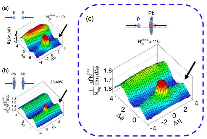
Two years ago, I reported the observation of surprising two-particle correlations at the CMS in proton-proton collisions, something that was previously observed at Brookhaven's RHIC in their 2005 gold-gold collisions.



You know that the LHC sometimes collides lead nuclei against lead nuclei instead of proton-proton pairs but a few weeks ago, it tried something something new, the proton-lead (asymmetric) collisions. Physics World tells us about a (not too) surprising result of this hybrid crashing game:

Unexpected 'ridge' seen in CMS collision data again

I wrote it's not "too" surprising because it's been seen in gold-gold, proton-proton, and lead-lead collisions, so why it should be missing in the proton-lead collisions? But there's something new about this story I haven't written about yet, and that's the reason for this new blog entry.

It's a new cute and plausible theoretical explanation of the ridge: color glass condensate.




Physics World refers to this fresh paper by a North Carolina-Brookhaven tandem:

Evidence for BFKL and saturation dynamics from di-hadron spectra at the LHC

BFKL stands for the Balitsky-Fadin-Kuraev-Lipatov equation which performs a resummation of \(\alpha_S \ln(x)\) terms that appear at each rung of the QCD ladder (here we really talk about Feynman diagrams that look like a ladder with rungs composed of QCD propagators: no kidding). For small \(x\), the right description is in terms of the so-called color glass condensate. You may try to read a funny 2006 paper by Frank Wilczek on the Origin of Mass; full text PDF as a basic background.

The color glass condensate is an interesting new state of matter – composed of quarks – that was proposed in 2000 and that is mathematically analogous to "spin glasses". There are several other cool ways to organize the quarks and their interactions that are intensely studied by some of the creative QCD folks. If I remember well, I learned about another one from a colloquium by Frank Wilczek in Massachusetts – it's called the color-flavor locking.

You know, this blog entry wasn't supposed to be too narrowly focused on the color glass condensate. It's about all similar amusing emergent concepts in QCD and the color-flavor locking is really pretty. ;-) What is it?

Before the color-flavor locking, its fathers have proposed another "behavioral mode" of the quarks in QCD, namely the following condensate (vacuum expectation value):\[

\langle q_i^\alpha C \gamma^5 q_j^\beta\rangle \propto \epsilon_{ij} \epsilon^{\alpha\beta 3}.

\] Here \(i,j\), the Latin indices, represent the flavor (up/down) while the Greek indices, \(\alpha,\beta\), encode the color. You see that the formula above picks the "third color" as a special one so \(SU(3)_c\) is broken to \(SU(2)_c\) while the chiral "flavor" \(SU(2)_L\times SU(2)_R\) group is unbroken.

But in the 1998 paper I have already mentioned, they proposed an even more natural condensate invariant under a "diagonal" \(SU(3)\), namely\[

\eq{
\langle q^\alpha_{Lia} q^\beta_{Ljb} \epsilon^{ab} \rangle &=
-\langle q^{\alpha\dot a}_{Ri} q^{\beta\dot b}_{Rj} \epsilon_{\dot a\dot b} \rangle=\\
&= \kappa_1 \delta_i^\alpha \delta_j^\beta +\kappa_2 \delta_j^\alpha\delta_i^\beta.
}

\] Note that there is no privileged "third color" in this formula. It uses the fact that there are three "pretty light" quark flavors, namely up/down/strange, and three colors. Of course, these two numbers "3" have nothing to do with each other – which is also why the Kronecker delta relating the Greek and Latin indices above is mixing apples and oranges. But because \(3=3\), it is actually possible to choose a random identification and use it to mix apples with oranges – and flavors with colors.

Originally, you had 1st, 2nd, 3rd flavor and 1st, 2nd, 3rd color. These two numbering systems had nothing to do with each other. That's also why you could have rotated the triplets by two independent \(SU(3)\) groups. If Nature ever makes you happy and creates a condensate given by the formula above, the numbering systems for the colors and flavors are identified by the "apple-orange" or "Latin-Greek" Kronecker delta symbols and only an overall \(SU(3)\) group which rotates the colors as well as flavors so that the Kronecker delta symbol is preserved – and these transformations that transform both "versions" of the \(SU(3)\) group in the same way are known as the diagonal group – are preserved symmetries.

Note that the equation above, claiming that the vacuum expectation value has a particular form, is a conjecture. They conjectured that in some situations, it may be true or at least approximately true. But if quarks ever organize themselves so that it is true, it has physical consequences. Alford, Rajagopal, and Wilczek decided that such a condensate would lead to various new "gaps" as well as new Nambu-Goldstone bosons that may be imagined as bound states of two quarks.

Because these "behavioral patterns for quarks" – color glass condensate or color-flavor locking – differ from the usual perturbative QCD that should hold at very short distances, as well as common descriptions of protons, neutrons, and other hadrons, they are considered extreme, perhaps even more extreme than the quark-gluon plasma. But they may have rather non-extreme properties and may be realized in various situations.

From the viewpoint of fundamental high-energy physics, experiments trying to find such exotic forms of nuclear matter are not searching for new physics. Even if those phases exist, they're just manifestations of the good old QCD. However, they are so new and "hard to rigorously calculate" manifestations of QCD that it's pretty interesting, anyway. QCD with colored and flavored quarks has quite some potential for various qualitatively different types of behavior so it's desirable for theorists to propose some initially weird conjectures about what the quarks and gluons could be doing, and for experimenters to check whether the predictions are ever realized.

The ridge seems to agree with some predictions from the color glass condensate and it's pretty interesting. But don't get carried away. Two years ago, I wrote that the ridge could be a sign of the quark-gluon plasma or the dual QCD string. People don't understand these signatures too accurately so the path from the observations to the right interpretations remains somewhat wiggly and shady.

CP violation

BTW, tonight, there will be a new paper on CP violation in D meson decays that will report a 3.5-sigma deviation from the Standard Model in a particular "difference of asymmetries" quantity seen in the 2011 LHCb data.

Different ways to interpret Feynman diagrams

Feynman diagrams are the funny pictures that Richard Feynman drew on his van:



You see that a Feynman diagram is composed of several lines that meet at vertices (at the nodes of the graph). Some of the lines are straight, some of them are wiggly: this shape of each line distinguishes the particle type. For example, straight lines are often reserved for fermions while wiggly lines are reserved for photons or other gauge bosons.




Some lines (I mean line intervals) are external – one of their two endpoints is free, unattached to anything. These are the external physical particles that must obey the mass on-shell condition \(p_\mu p^\mu = m^2\) and that specify the problem we're solving (i.e. what's the probability that some particular collection of particles with some momenta and polarization will scatter and produce another or the same collection particles with other momenta and polarizations). Other lines (I mean line intervals) are internal and they are unconstrained. You must sum over all possible ways to connect the predetermined external lines by allowed vertices and allowed internal lines. If you associate a momentum with these internal lines, also known as "propagators", it doesn't have to obey the mass on-shell condition. We say that the particle is "virtual". An explanation why its \(E\) may differ from \(\sqrt{p^2+m^2}\) is that the virtual particle only exists temporarily and the energy can't be accurately measured or imposed because of the inequality \(\Delta E\cdot\Delta t\geq\hbar/2\).

Because the virtual particles are not external, they define neither the initial state nor the final state. Still, they "temporarily appear" during the process, e.g. scattering, and they influence what's happening. In fact, they're needed for almost every interaction. Also, the Feynman diagrams have vertices at which several lines meet, where they terminate. The vertices describe the real events in the spacetime in which the particles merge, splht, or otherwise interact. However, we're doing quantum mechanics so none of these points in spacetime are uniquely or objectively determined. In fact, all the choices contribute to the calculable results – the total probability amplitudes.

A Feynman diagram is a compact picture that may be drawn by most kids in the kindergarten. However, each Feynman diagram – assuming we know the context and conventions – may also be uniquely translated to an integral, a contribution to the complex "probability amplitude" whose total value is used to calculate the probability of any process in quantum field theory. The laws used to translate the kindergarten picture to a particular integral or a related mathematical expression are known as the "Feynman rules".

How do we derive them?

I will discuss three seemingly very different methods:

• Dyson's series, an operator-based method
• Feynman's sum over histories i.e. configurations of fields
• Feynman's sum over histories i.e. trajectories of first-quantized particles

Richard Feynman originally derived his Feynman diagrams by the second method. As his name in the description of a method indicates, Freeman Dyson rederived the Feynman rules for the Feynman diagrams using the first method – and it was an important moment from a marketing viewpoint because this is how Freeman Dyson made Feynman diagrams extremely popular and essentially omnipresent.

The third method was added for the sake of conceptual completeness and it is the least rigorous one. However, it still gives you another way to think about the origin of Feynman diagrams – a way that is perhaps generalized in the "most straightforward way" if you try to construct Feynman diagrams for perturbative string theory.

It's important to mention that Feynman has discovered many things and methods, of course, but we shouldn't confuse them. The Feynman diagrams are the pictures on the van, tools to calculate scattering amplitudes and Green's functions. But he also invented the Feynman path integral ("sum over histories") approach to any quantum mechanical theory. It's not quite the same thing as the Feynman diagrams – it applies to any quantum theory, not just quantum field theory. However, as I have already said, he used the "sum over histories" of a quantum field theory to derive the Feynman diagrams for the first time.

Two other, conceptually differently looking ways to derive the Feynman diagrams were found later. The third method uses the "sum over histories" but applied to a "differently formulated system" than Feynman originally chose; the first method due to Dyson doesn't use the "sum over histories" at all.

Quadratic terms in the action, higher-order terms in the action

But all the three strategies to derive the Feynman rules share certain technical principles which are "independent of the formalism":

• The lines, both the propagators and the external lines, are associated with individual fields or particle species and with the bilinear or quadratic terms they contribute to the action (and the Lagrangian or the Hamiltonian).
• The vertices are associated with cubic, quartic, or other higher-order terms in the action (and the Lagrangian or the Hamiltonian), assuming that it is written in a polynomial form.

Let's assume we have an action and the Lagrangian that depends on the fields \(\phi_i\) in a polynomial way:\[

\eq{
\LL &= a_0 + \sum_i a_{1,i} \phi_i + \frac{1}{2!} \sum_{i,j} a_{2,ij} \phi_i\phi_j +\\
&+ \frac{1}{3!}\sum_{i,j,k} a_{3,ijk} \phi_i\phi_j\phi_k+\dots
}

\] which continues to higher orders, if needed, and which also contains various similar terms with the (first or higher-order) spacetime derivatives \(\partial_\mu\) of the fields \(\phi_i\) contracted in various ways. We don't consider the spacetime derivatives as something that affects the order in \(\phi\) so \(\partial_\mu \phi\partial^\mu \phi\) is still a second-order term in \(\phi\). The number of fields \(\phi_i\) – the order in \(\phi\) – that appear in the cubic or higher-order term will determine how many lines are attached to the corresponding vertex of the Feynman diagram.

The individual coefficients \(a_{n,i}\) etc. are parameters or "coupling constants" of a sort. How do we treat them?

Well, the first term, the universal constant \(a_0\), is some sort of the vacuum energy density. As long as we consider dynamics without gravity, it won't affect anything that may be observed. For example, the classical (or Heisenberg) equations of motion for the operators are unaffected because the derivative of a constant such as \(a_0\) with respect to any degree of freedom vanishes. We know that even in the Newtonian physics, the overall additive shift to energy is a matter of conventions. The potential energy is \(mgh\) where \(h\) is the height but you may interpret it as the weight above your table or above the sea level or above any other level and Newton's equations still work.

If we include gravity, the term \(a_0\) acts like a cosmological constant and it curves the spacetime. Fine. We will ignore gravity here so we will ignore \(a_0\), too.

The next terms are linear, proportional to \(a_{1,i}\). They are multiplied by one copy of a quantum field. For the Lorentz invariance to hold, it should better be a scalar field and if it is not, it must be a bosonic field and the vector indices must be contracted with those of some derivatives, e.g. as in \(\partial_\mu A^\mu\).

What do we do with the linear terms?

Well, here we can't say that they don't matter. They do depend on the fields and they do matter. But we will still erase them because of a different reason: they matter too much. If the potential energy contains a term proportional to \(\phi\) near \(\phi=0\), it means that \(\phi=0\) isn't a stationary point. The value of \(\phi\) will try to "roll down" in one of the directions to minimize the potential energy. It will either do so indefinitely, in which case the Universe is a catastrophically unstable hell, or it will ultimately reach a local minimum of the potential energy. In the latter, peaceful case, you may expand around \(\phi=\phi_{\rm min}\), i.e. around the new minimum, and if you do so, the linear terms will be absent.

So if we perform these basic steps, we see that without a loss of generality, we may assume that the Lagrangian only begins with the bilinear or quadratic terms. The following ones are cubic, and so on.

(We could start with a quantum field theory that has nontrivial linear terms, e.g. in the scalar field, anyway. In that case, the instability of the "vacuum" we assumed would manifest itself by a non-vanishing "one-point functions" for the relevant scalar field(s). The Feynman diagrams for these one-point functions ("scattering of a 1-particle state to a 0-particle state or vice versa") are known as "tadpoles" – tadpoles have a loop(s)/head and one external leg – because a journal editor decided that Sidney Coleman's alternative term for these diagrams, the "spermion", was even more problematic than a "tadpole".)

Bilinear terms and propagators

The method of Feynman diagrams typically assumes that we are expanding around a "free field theory". A free field theory is one that isn't interacting. What does it mathematically mean? It means that its Lagrangian is purely bilinear or quadratic. If we want to extract the "relevant" bilinear Lagrangian out of a theory that has many higher-order terms as well, we simply erase the higher-order terms.

Why is a quadratic Lagrangian defining a "free theory"? It's because by taking the variation, it implies equations of motions for the fields that are linear. And linear equations obey the superposition principle: if \(\phi_A(\vec x,t)\) and \(\phi_B(\vec x,t)\) are solutions to the equations of motion, so is \(\phi_A+\phi_B\). If \(\phi_A\) describes a wave packet moving in one direction and \(\phi_B\) describes a wave packet moving in another direction, they may intersect or overlap but the wave packets may be simply added which means that they pretend that they don't see one another: they just penetrate through their friend. This is the reason why they don't interact. Linear equations describe waves that just freely propagate and don't care about anyone else. Linear equations are derived from quadratic or bilinear actions. That's why quadratic or bilinear actions define "free field theories".

If we appropriately integrate by parts, we may bring the bilinear terms to the form\[

\LL_{\rm free}=\frac{1}{2}\sum_{ij} C_{ij} \phi_i P_{ij} \phi_j

\] where \(P_{ij}\) is some operator, for example \((\partial_\mu\partial^\mu+m^2)\delta_{ij}\). The factor \(1/2\) is a convention that is natural because if we differentiate the expression above with respect to a \(\phi_i\), we produce two identical terms due to the Leibniz rule for the derivative of the product. (That's not the case if the first \(\phi_i\) were \(\phi^*_i\) which is needed when it's complex: for complex fields, including the Dirac fields etc., the factor of \(1/2\) is naturally dropped.)

So the classical equations of motion derived for those fields look like this:\[

\sum_j P_{ij} \phi_j = 0.

\] You should imagine the Klein-Gordon equation as an example of such an equation.

Some operator, e.g. the box operator, acts on the fields and gives you zero. These are linear equations. You may often explicitly write down solutions such as plane waves, \(\phi_i = \exp(ip\cdot x)\), and all their linear superpositions are solutions as well. The coefficients of these plane waves are called creation and annihilation operators etc. You may derive what spectrum of free particles may be produced by a free field theory.

This may be done in the operator approach – the free fields are infinite-dimensional harmonic oscillators defined by their raising and lowering operators – as well as by the "sum over histories" approach – the harmonic oscillator may be solved in this way as well. The "sum over histories" approach encourages you to choose the \(\ket x\) or \(\ket{ \{\phi_i(\vec x,t)\} }\) continuous (or functionally metacontinuous) basis of the Hilbert space. By the functionally metacontinuous basis, I mean a basis that gives you a basis vector for each function or \(n\)-tuple of functions \( \{\phi_i(\vec x,t=t_0) \} \) even though these functions form a set that is not only continuous but actually infinite-dimensional.

But I want to focus on the derivation of the Feynman rules including the vertices. We don't want to spend hours with a free field theory. When we construct the Feynman rules, the free part of the action determines the particles that may be created and annihilated and that define the initial and final Hilbert space as a Fock space; and it determines the propagators.

The propagators will be determined by "simply" inverting the operator \(P_{ij}\) I used to define the bilinear action above. This inverted \(P^{-1}_{ij}\) plays the role of the propagator for a simple reason: we ultimately need to solve the linear equation of motion with some function on the right hand side. Each function may be written as a combination of continuously infinitely many (i.e. as an integral over) delta-functions so we really need to solve the equation\[

\sum_j P_{ij} \phi_j = \delta^{(4)} (x-x') \cdot k_i

\] for some coefficients \(k_i\) – which may be decomposed into Kronecker deltas \(\delta_{im}\) for individual values of \(m\). The value of \(x'\) – the spacetime event where the delta-function is localized – doesn't change anything profound about the equation due to the translational symmetry. A funny thing is that the equation above may be formally solved by multiplying it with the inverse operator:\[

\phi_i = \sum_j P^{-1}_{ij} \delta^{(4)}(x-x')\cdot k_j.

\] That's why the inverse of the operator \(P_{ij}\) – which is nonlocal (the opposite to differentiation is integration and we are generalizing this fact) appears in the Feynman rules.

So far I am presenting features of the results "informally"; we are not strictly deriving any Feynman rules and we haven't chosen one of the three methods yet.

Higher-order terms

I will postpone this point but the cubic and higher-order terms in the Lagrangian will produce the vertices of the Feynman diagrams. In the position representation, the locations of the vertices must be integrated over the whole spacetime.

In the momentum representation, the vertices are interactions that appear "everywhere" and we must instead impose the 4-momentum conservation at each vertex. In the latter approach, some momenta will continue to be undetermined even if the external particles' momenta are given. The more independent "loops" the Feynman diagram has, the more independent momenta running through the propagators must be specified. All the allowed values of the loop momenta must be integrated over.

The momentum and position approaches are related by the Fourier transform. Note that the Fourier transform of a product is a "convolution" and this is the sort of mathematical facts that translates the rules from the momentum representation to the position representation and vice versa.

Starting with the methods: Dyson series

We have already leaked what the final Feynman rules should look like so let us try to derive them. Dyson's method coincides with the tools in quantum mechanics that most courses teach you at the beginning, so it's a beginner-friendly method (although this statement depends on our culture and on those perhaps suboptimal ways how we teach quantum mechanics and quantum field theory). But it's actually not the first method by which the Feynman rules were derived; Feynman originally used the "sum over histories" applied to fields.

Dyson's method uses several useful technicalities, namely the Dirac interaction picture; time ordering; and a modified Taylor expansion for the exponential.

The Dirac interaction picture is a clever compromise between Schrödinger's picture in which the operators are independent of time and the state vector evolves according to Schrödinger's equation that depends on the Hamiltonian; and the Heisenberg picture in which the state vector is independent of time and the operators evolve according the Heisenberg equations of motion that resemble the classical equations of motion with extra hats (which are omitted on this blog because it's a quantum mechanical blog).

In the Dirac interaction picture, we divide the Hamiltonian to the "easy", bilinear part we have discussed above and this "free part" is used for the Heisenberg-like evolution equations (the operators evolve in a simple linear way as a result); and the "hard", higher-order or interacting part of the Hamiltonian which is used as "the" Hamiltonian in a Schrödinger-like equation. So we have:\[

\eq{
H(t) &= H_0 + V(t), \\
i\hbar \pfrac{\phi_i(\vec x,t)}{t} &= [\phi_i(\vec x,t),H_0]\\
i\hbar \ddfrac{\ket{\psi(t)}}{t} &= V(t)\ket{\psi(t)}.
}

\] The operators evolve according to \(H_0\), the free part, but the wave function evolves according to \(V(t)\). Note that \(V(t)\) – and of course the whole \(H(t)\) as well – is a rather general composite operator so it also depends on time: its evolution is also determined by its commutator with \(H_0\). On the other hand, \(H_0\) itself, while an operator, is \(t\)-independent because it commutes with itself.

The operator \(H_0\) depends on the elementary fields \(\phi_i\) in a quadratic way so the commutator in the second, Heisenberg-like equation above is linear in the fields \(\phi_i\). Consequently, these equations of motion are "solvable" and the solutions may be written as some combinations of the plane waves – the usual decomposition of operators \(\phi_i(\vec x,t)\) into plane waves multiplied by coefficients that are interpreted as creation and annihilation operators.

The proof that this Dirac interaction picture is equivalent to either Heisenberg or Schrödinger picture is analogous to the proof of the equivalence of the latter two pictures themselves; one just considers "something in between them".

Getting the time-ordered exponential

At any rate, we may now ask how the initial state \(\ket\psi\) at \(t=-\infty\) evolves to the final state at \(t=+\infty\) via the Schrödinger-like equation that only contains the interacting (higher-order) \(V(t)\) part of the Hamiltonian. We may divide the evolution into infinitely many infinitesimal steps by \(\epsilon\equiv \Delta t\). The evolution in each step (the process of waiting for time \(\epsilon\)) is given by the map\[

\ket\psi \mapsto \zav{ 1+\frac{\epsilon}{i\hbar} V(t) }\ket\psi.

\] For an infinitesimal \(\epsilon\), the terms that are higher-order in \(\epsilon\) may be neglected. To exploit the formula above, we must simply perform this map infinitely many times on the initial \(\ket\psi\). Imagine that one day is very short and its length is \(\epsilon\) and use the symbol \(U_t\) for the parenthesis \(1+\epsilon V(t)/i\hbar \) above. Then the evolution over the first six days of the week will be given by\[

\ket\psi \mapsto U_{\rm Sat} U_{\rm Fri} U_{\rm Thu} U_{\rm Wed} U_{\rm Tue} U_{\rm Mon}\ket\psi.

\] Note that the Monday evolution operator acts first on the ket, so it appears on the right end of the product of evolution operators. The later day we consider, the further on the left side – further from the ket vector – it appears in the product. So the evolution from Monday to Saturday (or Sunday) is given by a product where the later operators are always placed on the left side from the earlier ones. We call such products of operators "time-ordered products".

In fact, we may define a "metaoperator" of time-ordering \({\mathcal T}\) which, if it acts on things like \(V(\text{Day1}) V(\text{Day2})\), produces the product of the operators in the right order, with the later ones standing on the left. The ordering is important because operators usually refuse to commute with each other in quantum mechanics.

Now, if you study the product of the \(U_{\rm Day}\) operators above, you will realize that the product generalizes our favorite "moderate interest rates still yield the exponential growth at the end" formula for the exponential\[

\exp(X) = \lim_{N\to \infty} \zav{ 1 + \frac XN }^N

\] where \(1/N\) may be identified with \(\epsilon\). The generalization affects two features of this formula. First, the terms \(X/N\) aren't constant, i.e. independent of \(t\), but they gradually evolve with \(t\) because they depend on \(V(t)\). Second, we mustn't forget about the time ordering. Both modifications are easily incorporated. The first one is acknowledged by writing \(X\) inside \(\exp(X)\) as the integral over time; the second one is taken into account by including the "metaoperator" of time-ordering. (I call it a "metaoperator" so that it suppresses your tendency to think that it's just an operator on the Hilbert space. It's not. It's an abstract symbol that does something with genuine operators on the Hilbert space. What it does is still linear – in the operators.)

With these modifications, we see that the evolution map is simply\[

\ket\psi\mapsto {\mathcal T} \exp\zav{ \int_{-\infty}^{+\infty}\dd t\, \zav{ \frac{V(t)}{i\hbar} } } \ket\psi

\] The time-ordered exponential is an explicit form for the evolution operator (the \(S\)-matrix) that simply evolves your Universe from minus infinity to plus infinity. In classical physics, you could rarely write such an evolution map explicitly but quantum mechanics is, in a certain sense, simpler. Linearity made it possible to "solve" the most general system by an explicit formula.

Once we have this "time-ordered exponential", we may deal with it in additional clever ways. The exponential may be Taylor-expanded, assuming that we don't forget about the time-ordering symbol in front of all the monomial terms in the Taylor expansion. The operators \(V(t)\) are polynomial in the fields and their spacetime derivatives: we allow each "elementary field" factor to either create or annihilate particles in the initial or final state (these elementary fields will become the inner end points of external lines of Feynman diagrams); or we keep the elementary fields "ready to perform internal services". In the latter case, we will need to know the correlators such as\[

\bra 0 \phi_i(\vec x,t) \phi_j(\vec x', t')\ket 0

\] which is a sort of a "response function" that may be calculated – even by the operator approaches – and which will play the role of the propagators. The remaining coefficients and tensor structures seen in \(V(t)\) will be imprinted to the Feynman rules for the vertices, the places where at least 3 lines meet.

I suppose you know these things or you will spend enough time with the derivation so that you understand many subtleties. My goal here isn't to go through one particular method in detail, however. My goal is to show you different ways how to look at the derivation of the Feynman diagrams. They seem conceptually or philosophically very different although the final predictions for the probability amplitudes are exactly equivalent.

Feynman's original method: "sum over histories" of fields

Feynman originally derived the Feynman rules by "summing over histories" of fields. The very point of the "sum over histories" approach to quantum mechanics is that we consider a classical system, the classical limit of the quantum system we want to describe, and consider all of its histories, including (and especially) those that violate the classical equations of motion. For each such a history or configuration in the spacetime, we calculate the action \(S\), and we sum i.e. integrate \(\exp(iS/\hbar)\) over all these histories, perhaps with the extra condition that the initial and final configurations agree with the specified ones (those that define the problem we want to calculate).

(See Feynman's thesis: arrival of path integrals, Why path integrals agree with the uncertainty principle, and other texts about path integrals.)

We have already mentioned that we're dividing the action, Lagrangian, or Hamiltonian to the "free part" and the "interacting part". We're doing the same thing if we use this Feynman's original method, too. To deal with the external lines, we have to describe the wave functions (or wave functionals) for the multiparticle states; this task generalizes the analogous problem with the quantum harmonic oscillator to the case of the infinite dimension and I won't discuss it in detail.

What's more important are the propagators, i.e. the internal lines, and the vertices. The propagators produce the inverse operator \(P_{ij}^{-1}\) from the Lagrangian again. These "Green's functions" have the property I have informally mentioned – they solve the "wave equation" with the Dirac delta-function on the right hand side; and they are equal to the two-point correlation functions evaluated in the vacuum.

But Feynman's path integral has a new way to derive the appearance of this inverse operator as the propagator. It boils down to the Gaussian integral\[

\int \dd^n x\,\exp(\vec x\cdot M\cdot \vec x) = \frac{\pi^{n/2}}{\sqrt{\det M}}.

\] but what is even more relevant is a modified version of this integral that has an extra linear term in the exponent aside from the bilinear piece:\[

\int \dd^n x\,\exp(\vec x\cdot M\cdot \vec x+ \vec J\cdot \vec x) = \dots

\] This more complicated integral may be solved by "completing the square" i.e. by the substitution\[

\vec x = \vec x' - \frac{1}{2} M^{-1}\cdot \vec J.

\] With this substitution, after we expand everything, the \(\vec x'\cdot \vec J\) "mixed terms" get canceled. As a replacement, we produce an extra term\[

-\frac{1}{4} \vec J\cdot M^{-1} \cdot \vec J

\] in the exponent; the coefficient \(-1/4\) arises as \(+1/4-1/2\). And because \(M\) is the matrix that is generalized by our operator \(P_{ij}\) discussed previously, we see how the inverse \(P^{-1}_{ij}\) appears sandwiched in between two vectors \(\vec J\).

The strategy to evaluate the Feynman's path integral is to imagine that this whole integral is a "perturbation" of a Gaussian integral we know how to calculate. We work with all the \(V(\vec x,t)\) interaction terms as if they were general perturbations similar to the \(\vec J\) vector above, and in this way, we reproduce all the vertices and all the propagators again.

Note that I have been even more sketchy here because this text mainly serves as a remainder that there exists a "philosophically different attitude" to the Feynman diagrams that one shouldn't overlook or dismiss just because he got used to other techniques and a different philosophy. If you want to calculate things, it's good to learn one method and ignore most of the others so that you're not distracted. But once you start to think about philosophy and generalizations, you shouldn't allow your – often random and idiosyncratic – habits to make you narrow-minded and to encourage you to overlook that there are completely different ways how to think about the same physics. These different ways to think about physics often lead to different kinds of "straightforward generalizations" that might look very unnatural or "difficult to invent" in other approaches.

In science, one must disentangle insights that are established – directly or indirectly supported by the experimental data – from arbitrary philosophical fads that you may be promoting just because you got used to them or for other not-quite-serious reasons. Of course, this broader point is the actual important punch line I am trying to convey by looking at a particular technical problem, namely methods to derive the Feynman rules.

Feynman's other method: "sum over histories" of merging and splitting particles

Once I have unmasked my real agenda, I will be even more sketchy when it comes to the third philosophical paradigm. You may "derive" the Feynman rules, at least qualitatively, from the "first-quantized approach" emulating non-relativistic quantum mechanics.

Again, in this derivation, we are "summing over histories". But they're not "histories of the fields \(\phi_i(\vec x,t)\)" as in the approach from the previous section – the original method Feynman exploited to derive the Feynman rules. Instead, we may sum over histories of ordinary mechanics, i.e. over histories of trajectories \(\vec x(t)\) for different particles in the process.

This approach, emulating non-relativistic quantum mechanics, the propagators \(D(x,y)\) arise as the probability amplitude for a particle to get from the point \(x\) of the spacetime to the point \(y\). It just happens that the form of the propagators – which have been interpreted as matrix elements of the "inverse wave operator" \(P^{-1}_{ij}\); and as two-points functions evaluated in the vacuum – may also be interpreted as the amplitude for a particle getting from one point to another.

Well, this works in some approximations and one needs to deal with antiparticles properly in order to restore the Lorentz invariance and causality (note that the sum over particles' trajectories still deals with trajectories that are superluminal almost everywhere, but the final result still obeys the restrictions and symmetries of relativity!) and it's tough. At the end, the "derivation" ends up being a heuristic one.

But morally speaking, it works. In this interpretation, a Feynman diagram encodes some histories of point-like particles that propagate in the spacetime and that merge or split at the vertices which correspond to spacetime points at which the total number of particles in the Universe may change (this step would be unusual in non-relativistic quantum mechanics, of course). The path integral over all the paths of the internal particles gives us the propagators; the vertices where the particles split or join must be accompanied by the right prefactors, index contractions, and other algebraic structures. But in some sense, it works.

It's this interpretation of the Feynman diagrams that has the most straightforward generalization in string theory. In string theory, we may imagine cylindrical or strip-like world sheets – histories of a single closed string or a single open string propagating in time – and they generalize the world lines. The path integral over all histories like that, between the initial closed/open string state and the final one, gives us a generalized Green's function for a single string.

And in string theory, we simply allow the topology of the world sheet to bd nontrivial – to resemble the pants diagram or the genus \(h\) surface with additional boundaries or crosscaps – and it's enough (as well as the only consistent way) to introduce interactions. While the interactions of point-like particles are given by vertices, "singular places" of the Feynman diagrams, and this singular character of the vertices is ultimately responsible for all the short-distance problems in quantum field theories, the world sheets for strings have no singular places at all. They're smooth manifolds – each open set is diffeomorphic to a subset of \(\RR^2\), especially if you work in the Euclidean signature – but if you look at a manifold globally (and only if you do so), you may determine its topology and say whether some interactions have taken place.

So this third method of interpreting the Feynman diagrams – as the sum over histories of point-like particles in the spacetime that are allowed to split and join at the vertices – which was the "most heuristic one" and the "method that was least connected to exact formulae" encoding the mathematical expressions behind the Feynman diagrams actually becomes the most straightforward, the most rigorous way to derive the analogous amplitudes in string theory.



Take the world from another point of view, interview with RPF, 36 minutes, PBS NOVA 1973. At 0:40, he also mentions that brushing your teeth is a superstition. Given my recent appreciation of the yeasts that are unaffected by the regular toothpastes, I started to think RPF had a point about this issue, too.

If you got stuck with a particular "philosophy" how to derive the Feynman rules, e.g. with Dyson's series, it could be much harder – but not impossible – to derive the mathematical expressions for multiloop string diagrams. There have been many methods due to Richard Feynman mentioned in this text but once again, the most far-reaching philosophical lesson is one that may be attributed to Richard Feynman as well:

Perhaps Feynman's most unique and towering ability was his compulsive need to do things from scratch, work out everything from first principles, understand it inside out, backwards and forwards and from as many different angles as possible.

I took the sentence from a review of a book about Feynman. It's great if you decompose things to the smallest possible blocks, rediscover them from scratch, and try to look at the pieces out of which the theoretical structure is composed from as many angles as you can. New perspectives may give you new insights, new perceptions of a deeper understanding, and new opportunities to find new laws and generalize them in ways that others couldn't think of.

And that's the memo.

P.S.: BBC and Discovery's Science Channel plan to shoot a Feynman-centered historical drama about the Challenger tragedy.



Prayer for Marta ["Let the peace remain with this land. Let anger, envy, jealousy, fear and conflicts subside, let them subside. Now when your lost control over your things will return to you, the people, it will return to you..."], an iconic politically flavored 1968 song by which the singer restarted freedom lost in 1968 during the Velvet Revolution in 1989.

P.P.S.: Ms Marta Kubišová, a top Czech pop singer in the late 1960s (Youtube videos), refused to co-operate with the pro-occupation establishment after the 1968 Soviet invasion which is why she became a harassed clerk in a vegetable shop rather than a pillar of the totalitarian entertainment similar to her ex-friend Ms Helena Vondráčková.

She just received Napoleon Bonaparte's Legion of Honor award, a well deserved one. Congratulations!

Preons probably can't exist

Don Lincoln is the star of several cute Fermilab videos in which he explains various issues in particle physics. He's also authored several related texts for Fermilab Today.



He chose a much more controversial topic, namely preons, for his fresh article in the Scientific American:

The Inner Life of Quarks

Preons are hypothetical particles smaller than leptons and quarks that leptons and quarks are made out of. But can there be such particles?




At first sight, the proposal seems natural and may be described by the word "compositeness". Atoms were not indivisible, as the Greek word indicated, but they had smaller building blocks – the nucleus and the electron. The nuclei weren't indivisible, either – they had protons and neutrons inside. The protons and neutrons weren't indivisible – they have quarks inside.

Why shouldn't this process continue? Why shouldn't there be smaller particles inside quarks? Or inside the electron and other leptons?

Many people who pose this question believe that it is a rhetorical question and they don't expect any answer. Instead, they overwhelm you with detailed speculations `bout the possible composition of quarks and leptons while they possess lots of wishful thinking when they believe that all the problems they encounter are just details that can be overcome.

(Pati and Salam introduced preons for the first time in 1974. One of the other early enough particular realizations of preons were "rishons" by Harari, Shupe, and a young Seiberg, which means "primary" in Hebrew. I guess that prazdrojs and urquells would be the Czech counterparts. The terminology describing preons has been much more diverse than the actual number of promising ideas coming from this research. The names for "almost the same thing" have included prequarks, subquarks, maons, alphons, quinks, Rishons, tweedles, helons, haplons, Y-particles, and primons.)

However, the question above is a very good, serious question and it actually has an even better answer that explains why.

Mass scales and length scales

Since the mid 1920s and realizations due to Louis de Broglie, Werner Heisenberg, and a few others, we've known about a fundamental relationship between the momentum of a particle and the wavelength of a wave that is secretly associated with it:\[

\lambda = \frac{2\pi \hbar}{p}.

\] You may use units of mature particle physicists in which \(\hbar=1\). In those units, you may omit all factors of \(\hbar\) because they're equal to one and the momentum has the same dimension as the inverse length. Note that adult physicists also tend to set \(c=1\) because the speed of light is such a natural "conversion factor" between distances and times that has been appreciated since Einstein's discovery of special relativity in 1905.

In those \(\hbar=c=1\) units, energy and momentum (and the mass) have the same units, and space and time have the same units, too. The first group is inverse to the second group. Particle physicists love to use \(1\GeV\) for the energy (and therefore also momentum and mass); the inverse \(1\GeV^{-1}\) is therefore a unit for distances and times. One gigaelectronvolt is approximately the rest mass of the proton, slightly larger than the kinetic and potential energies of the quarks inside the proton; the inverse gigaelectronvolt interpreted as a distance is relatively close to the radius of the proton.

At any rate, the de Broglie relationship above says that the greater momentum a particle has, the shorter the wave associated with it is. Similarly, the periodicity of the wave obeys\[

\Delta t = \frac{2\pi\hbar}{E}

\] where \(E\) is the energy. The phase of the wave returns to the original value after a period of time that is inversely proportional to the energy. Now, it is sort of up to you whether \(E\) is the total energy that contains the latent energies \(E=mc^2\) or whether these terms are removed. If you want a fully relativistic description and you're ready to create and annihilate particles, you obviously need to include all the terms such as \(E=mc^2\).

On the other hand, if you study a non-relativistic system, it may be OK to remove \(E=mc^2\) from the total energy and consider \(mv^2/2\) to be the leading kinetic contribution to the energy. That's how we're doing it in non-relativistic quantum mechanics. These two conventions differ by a time-dependent reparameterization of the phase of the wave function (which isn't observable),\[

\psi_\text{relativistic}(\vec x,t) = \psi_\text{non-relativistic}(\vec x,t) \cdot \exp(-i\cdot Mc^2\cdot t/ \hbar)

\] where \(M\) is the total rest mass of all the particles. The relativistic wave function's phase is just rotating around much more quickly than the non-relativistic one.

Preons don't explain any patterns

Fine. Let's return to compositeness and preons. When you conjecture that leptons and quarks have a substructure, you want this idea to lead to exciting consequences. For example, you want to explain why there are many types (flavors) of leptons and quarks out of a more economic basic list of preonic building blocks. It's not a necessary condition for preons to exist but it would be nice and sort of needed for the idea to be attractive.

This goal doesn't really work with preons. Note that it did work with quarks; that's how Gell-Mann discovered or invented quarks. There were many hadrons and the idea that all these particles were composed of quarks was actually able to explain a whole zoo of hadrons – particles related to the proton and neutron, including these two – out of a more economic list of types of quarks.

Gell-Mann's success can't really be repeated with the preons. The list of known leptons and quarks is far from "minimal" but it is not sufficiently complicated, either. Quarks have three colors under \(SU(3)_c\). And both leptons and quarks are typically \(SU(2)_W\) doublets. And both leptons and quarks come in three generations.

These are three ways in which there seems to be a "pattern" in the list of types of quarks and leptons; three directions in which the lists of quarks and leptons seem to be "extended". But none of them may be nicely explained by preons. First, you can't really explain why there are \(SU(2)_W\) doublets or \(SU(3)_c\) triplets. Whatever elementary particles you choose, they must ultimately carry some nonzero \(SU(2)_W\) and \(SU(3)_c\) charges – and the charges of the doublets and triplets are really the minimal ones (the simplest representations) so whatever the preons are, they can't really be simpler than quarks or leptons.

(Here I am assuming that the gauge bosons and gauge fields aren't "composite". The possibility of their compositeness is related to preons and the discussion why it's problematic would be similar to this one but it would differ in some important details. The conclusion is that composite gauge bosons are even more problematic than preons.)

Also, you won't be able to produce three families out of a "simpler list of preons". To produce exactly three families, you need something that comes in three flavors, i.e. a particle of "pure flavor" that has three subtypes and that binds to other particles to make them first- or second- or third-generation quarks or leptons. But there must still be other particles that carry the weak and strong charges so the result just can't be simpler.

The comments above were really way too optimistic. The actual problems with the "diversity of the bound states" that you get out of preons are much worse. Much like there are hundreds of hadron species, you typically predict hundreds of bound states of preons. Moreover, they should allow multiple arrangements of the preons' spins, they should be ready to be excited, and they should produce much more structured bound states. None of these things is observed and the predicted structure just doesn't seem to have anything to do with the observed, rather simple, list of quark and lepton species.

But there exists a problem with preons that is even more serious: their mass.

If it makes any sense to talk about them as new particles, they must have some intrinsic rest mass, much like quarks and leptons. What can the mass be? We may divide the possibilities to two groups. The masses may either be smaller than \(1\TeV\) or greater than \(1\TeV\). I chose this energy because it's the energy that is slightly smaller than the LHC beams and that is already "pretty nicely accessible" by the LHC collider. Maybe I should have said \(100\GeV\) but let's not be too picky.

If the new hypothetical preons are lighter than \(1\TeV\), then the new hypothetical particles are so light that the LHC collider must be producing them rather routinely. If that were so, they would add extra bumps and resonances and corrections and dilution to various charts coming from the LHC. Those graphs would be incompatible with the Standard Model that assumes that there are no preons, of course. But it's not happening. The Standard Model works even though it shouldn't work if the preons were real and light.

So we're left with the other possibility, namely that preons are heavier than \(1\TeV\) or \(100\GeV\) or whatever energy similar to the cutting-edge energies probed by the LHC these days. But that's even worse because the very purpose of preons is to explain quarks and leptons as bound states of preons – and the known quarks and leptons are much lighter than \(1\TeV\).

To get a \(100\MeV\) strange quark, to pick a random "mediocre mass" example, the rest mass of preon(s) inside the quark, several \(\TeV\), would have to be almost precisely cancelled by other contributions to the mass and energy, with the accuracy better than 1 in 10,000. Clearly, the extra terms can't be kinetic energy which is positively definite: the compensating terms would have to be types of negative (binding) potential energy.

But it's extremely unlikely for the energy to be canceled this accurately, especially if you expect that the cancellation holds for many different bound states of preons (because many quarks and leptons are light).

Note that the virial theorem tells us that in non-relativistic physics, it's normal that the kinetic energy and the potential energy are of the same order. For example, for the harmonic oscillator with the \(kx^2/2\) potential energy, the average kinetic energy and the average potential energy are the same. For the Kepler/Coulomb problem, \(V\sim - k/r\), and the kinetic energy is \((-1/2)\) times the (negative) potential energy. More generally,\[

2\langle E_{\rm kin}\rangle = -\sum_{m=1}^N \langle \vec F_m\cdot \vec r_m\rangle

\] and if the potential goes like \(V\sim k r^n\), then \[

\langle E_{\rm kin} \rangle =\frac{n}{2} \langle V\rangle.

\] If you need the potential energy to cancel, you have to assume \(n=-2\). But the attractive potentials \(-1/r^2\) are extremely unnatural in 3+1 dimensions where \(-1/r\) is the only natural solution to the Poisson-like equations you typically derive from quantum field theories. You won't be able to derive them from any meaningful theory. Moreover, relativistic corrections will destroy the agreement even if you reached one. I was assuming that the motion of preons may be represented by non-relativistic physics – because the preons are pretty heavy and at relativistic speeds, they would be superheavy. If you assume that they're heavy and relativistic (near the speed of light), you will face an even tougher task to compensate their relativistically enhanced kinetic energy.

Even if you fine-tuned some parameters to get a cancellation, it will probably not work for other preon bound states. The degree of fine-tuning needed to obtain many light bound states is probably amazingly high. And we're just imposing a few conditions – the existence of light bound states that may be called "leptons and quarks". We should also impose all other known conditions – e.g. the non-existence of all the other bound states that the preon model could predict and the right interactions of the bound states with each other and with other particles – and if we do so, we find out that our problems are worse than just a huge amount of fine-tuning. We simply won't find any working model at all even if we're eager to insert arbitrarily fine-tuned parameters.

If you think about the arguments above, you are essentially learning that you shouldn't even attempt to explain light elementary particles – those that are lighter than the energy frontier, e.g. the energy scale that is being probed by the current collider – as composites. It can never really work. Quarks and leptons are much lighter than the LHC beam energy and because no sign of compositeness (involving new point-like particles) has been found, it really means that there can't be any.

Compositeness has done everything for us

So while the idea of compositeness is responsible for many advances in the history of physics, nothing guarantees that such "easy steps" may be done indefinitely. In fact, it seems likely that there won't be another step of this sort although some bold proposals that the top quark etc. could still be composite exist and are marginally compatible with the known facts.

After all, wouldn't you find it painful if the progress in physics were reduced to repeating the same step "our particles are composed of even smaller ones" that you would repeatedly and increasingly more mechanically apply to the current list of particles? The creativity in physics would be evaporating.

There exists a sense in which quarks and leptons are composite and the counter-arguments above are circumvented. In string theory, a lepton or a quark is a string. That means that you may interpret each such elementary particle as a bound state of "many string bits", pearls or beads along the string. If the number of conjectured "smaller building blocks" becomes infinite, like it is in the case of the stringy shape of an elementary particle, the cancellation between the kinetic and potential energy may become totally natural.

Despite the inner structure of elementary particles, string theory has an explanation why there are massless (or approximately massless, in various approximations) particles in the stringy spectrum. To some extent, this masslessness is guaranteed by having the "critical spacetime dimension" \(D=10\) or \(D=26\) for the superstring and bosonic string case, respectively. Well, string theory circumvents another problem we mentioned, too. We said that the kinetic energy is positive and the sum of all such positive terms must be positive, too. However, string theory uses the important fact that the sum of all positive integers equals \(-1/12\) which provides us with a very natural opportunity to cancel infinitely many terms although all of them seem to be positive.

Comparing preons and superpartners

The LHC hasn't found traces of any new particles beyond those postulated by the Standard Model of particle physics yet. However, that doesn't mean that all proposals for new physics are in the same trouble. In particular, I think it's important to explicitly compare preons with superpartners predicted by the supersymmetry.

At some point in the discussion above, I mentioned that preons could be either lighter or heavier than \(1\TeV\). The case of "light new particles" is generally excluded by the LHC (and previous experiments) because we would have already produced these new particles if they existed and if they were light.

The case of preons heavier than \(1\TeV\) was problematic because their "already high mass" must have been accurately cancelled by some negative contributions to the total energy/mass of the bound states and the negative potential energy required to do so seemed impossible, fine-tuned, and generally hopeless.

But the case of superpartners heavier than \(1\TeV\) doesn't have any problems of this sort. No supersymmetry phenomenologist really has any "rock solid" argument of this sort that would imply that the gluino is lighter than \(1\TeV\) or heavier than \(1\TeV\). We just don't know, these new particles may be discovered at every moment, and even at several \(\TeV\) or so, they still immensely improve the situation with the fine-tuning of the Higgs mass etc.

So while preons are pretty much completely dead – because you just can't construct light particles out of heavy ones, if I oversimplify just a tiny bit – superpartners remain immensely viable and well-motivated. The superpartners may still be rather light – the lower bound on their mass are often significantly lower than the lower bounds on other particles' masses in models of new physics – but there's nothing wrong about their being much heavier, either.

Much like in many texts, it's important not to become a dogmatic advocate of some ideas you decide to "love" in the first five minutes of your research. You could fall in love with the preons. Except that if you impartially study them in much more detail, you find out that this paradigm doesn't really agree with the known features of the world of particles well and some clever enough arguments may actually exclude rather vast and almost universal classes of such models. You should never become a blinded advocate of a theory who becomes blind to arguments of a certain type, e.g. the negative ones that unmask a general disease of your pet theory.

Preons are pretty much hopeless while other models of new physics remain extremely well motivated and promising.

And that's the memo.



P.S.: There will be a Hadron Collider Physics HCP 2012 conference in Kyoto in two weeks; see some of the ATLAS talks under HCP-2012. The detectors should update some of their data from 5 to 12+ inverse femtobarns of the 2012 data which means from 10 to 17 inverse femtobarns of total data. It's just a 30% improvement in the accuracy. Expect much more in March 2013 in Moriond.



Also, Czechia celebrates the main national holiday today, the anniversary of the 1918 birth of Czechoslovakia.

Alan Guth on himself, science, cosmology

Aside from Edward Witten, another well-known winner of the Newton Medal (in 2009) was Alan Guth, the first father of cosmic inflation. Two month ago, the Institute for Physics posted the post-Newton-Medal interview with him, too.



He had no science background in his family. At least he doesn't remember any background. But his family was happy when it learned that Alan was into science. Well, they were happy for a while, before they realize that science wasn't quite the same thing as engineering, but it was fortunately too late for them intervene. ;-)

He grew up in a small town, Highland Park, New Jersey which only has 15,000 inhabitants or so today. Well, it may be a small town but your humble correspondent knows it very well from his Rutgers years (1997-2001). In fact, I officially had a physician over there although I have never visited him so at least, I was sometimes going to do shopping in a grocery store over there. You may guess what Guth's father was: Yes, he had a grocery store in Highland Park. It burned at some point. ;-)




Many or most people in the Academia and especially theoretical physics come from scholarly families – the tradition usually goes back several generations, in fact. It has advantages and it has disadvantages. This "inherited occupation" adds some amount of sterility to the environment. On the other hand, the "scholars who inherited the job" are trained to be productive scholars so I am pretty sure that in average, they write many more papers than the "first explorers of the scientific occupation in a family". The latter may often be more audacrious and creative, however.

Guth was affected by a fabulous high school teacher. He didn't know too much physics, Alan Guth later realized, but he was still lucky to have a dynamic guy of this type. He described some success of him as a theoretical physics when he was a high school pupil – something based on a pure thought but it still works well. ;-) Alan Guth married his high school sweetheart. Two kids, the son is a mathematician who proved e.g. the Son-of-Guth Theorem (naming convention due to Susskind, if I caught it well).

MIT was where he went to college. MIT was unusual socially because it didn't separate people who are "in" and "out". He liked it. He was surprised he had superior competitors – unthinkable at the high school. People specialized a bit. He became sure he wanted to be a theoretical physicist. Grad school. Postdoc jobs. One of them made him interested in cosmology. Magnetic monopoles in the early Universe became his important obsession.

Alan Guth explains what cosmology is – science of the Universe as a whole, especially focusing on its childhood. The Big Bang Theory was great but it needed things to be fine-tuned and failed to explain the uniformity, too. He discovered cosmic inflation while solving another problem, namely why Sheldon Cooper of The Big Bang Theory has't found magnetic monopoles during their polar expedition. Guth explains why inflation gives the bang to the Big Bang. A gram of matter is enough to create our large visible Universe. A gram is not much but it's still much more than the Planck mass so it's not a theory of everything.

It looked dramatic so he was afraid it was wrong but after some talks, especially those with big shots in the audience, it became clear it wasn't wrong. Today, cosmology is in the golden age, indeed. Things are accurate. He describes the composition of the Universe and the absolute nothingness at the beginning. God is pointless because because He is just a redundant connecting link – with this addition, you must just explain why He is there instead of the Universe. ;-)

Hat tip: Joseph S.

Edward Witten on science, strings, himself

Two months ago, the Institute of Physics revealed this YouTube video:



Edward Witten, whom they still call "a 2010 Newton Medal Winner" rather than the "An Inaugural Milner Prize Winner" because they think that £1,000 with a stamp "IOP" on it (plus the name of Isaac Newton, without his permission) is more than $3,000,000 ;-), is talking for 25 minutes about his CV, previous scholarly interests, as well as hot topics in string theory.




Edward Witten is known for having studied some social sciences – journalism, history, linguistics – and being a tool of the Democratic Party candidates (such as George McGovern 1972 who just died) but he has been interested in physical sciences from his childhood. He was interested in astronomy but he was afraid that the job required him to be an astronaut. It is cute to mix astronomers and astronauts. My dad doesn't distinguish astronomers from astrologers.

Of course, his father – a theoretical physicist – was probably affecting Edward Witten, too.

He has been interested in the peace in the Middle East. In fact, some of his $3 million Milner money is going to J Street, a left-wing NGO trying to create peace between the Israeli Arabs and Jews in some of the most naive ways. Of course, just like anyone who takes string theory seriously, he shows an old picture of himself on a camel.

He talks about his wife, kids, and interests. His parents didn't believe in pushing kids too far too quickly. He got a standard theoretical physics education rather soon. Only when he was a postdoc, his maths was getting deeper. Supersymmetry became essential when he was a student. It has played a key role in his research from the beginning.

Some extra remarks are dedicated to Einstein's general relativity, extra dimensions, and unification of all forces. He talks about his negative-energy instability of higher dimensions without SUSY. He paints himself as a relative latecomer to string theory. Of course, it depends whom you compare him with. Witten compares the beauty of the sound of different musical instruments depending on the admixtures of the higher Fourier modes.

In the early 1980s, he realized that the available consistent string vacua failed to violate the left-right symmetry (P and CP). At some moment in 1984, the first superstring revolution explodes and it was the first string miracle that occurred when Witten was watching. That's why it was a signal from the Heaven for him. String theory got much more realistic.

The 1990s are the decade of dualities and M-theory. Who needed the other four string theories, and so on. From that time, he's been intrigued by the application of string/M-theoretical methods to understand issues in "ordinary" established particle physics theories (why positive energy, why confinement, ...). This light that string theory manages to shine upon the established theories is Witten's main reason to be convinced that string theory is on the right track. The elegance with which string theory sheds the light is another reason. Witten still calls our understanding of string theory "the rough draft" but this rough draft has already led to amazing insights and Witten doesn't believe that such a chain of astonishing discoveries has happened by coincidence.

The last reason why string theory seems right to him is that it teaches us new and deeper things about the geometry – including things that surprised mathematicians and inspired those at the frontier. He hadn't expected such a thing when he was young but these insights did materialize. Our confusion has actually helped to develop the new concepts.

A special discussion is dedicated to the big mystery what is the core principle underlying string theory much like the equivalence principle or spatial curvature underlying Einstein's general relativity. What string theory really means? It fascinates him most. But for decades, the theory has been smarter than us and forced us to move in previously unanticipated direction with twists – and that's probably still true today.

Witten isn't actively trying to solve the biggest questions. He says a thing often told by Andy Strominger as well – an important skill in the research is to choose a question small enough so that you have a chance to answer it but big enough so that it is worth answering. The Khovanov issues are mentioned as an example. Witten couldn't understand what the stuff was about – but he did understand it was physics-related (I am not that far). Witten makes it clear he realizes that most string theorists aren't interested in those things but he's independent enough not to care. Of course, there's no guarantee this stuff will be important. He knows that but he suspects it will be important. ;-)

At the end, he compares the string theory research with the discovery of new continents and with finding a treasure underground that we don't fully understand but we see that pieces fit together.

New element

Some fun via Fred S. – a new densest element was just found.