When truths don't commute. Inconsistent histories.

A short introduction to Consistent Histories after some trivial appetizer

When the uncertainty principle is being presented, people usually – if not always – talk about the position and the momentum or analogous dimensionful quantities. That leads most people to either ignore the principle completely or think that it describes just some technicality about the accuracy of apparatuses.

However, most people don't change their idea what the information is and how it behaves. They believe that there exists some sharp objective information, after all. Nevertheless, these ideas are incompatible with the uncertainty principle. Let me explain why the uncertainty principle applies to the truth, too.




Every proposition we can make about objects in Nature and their properties may be determined by a measurement and mathematically summarized as a Hermitian projection operator \(P\),\[

P = P^\dagger, \quad P^2=P.

\] The first condition is the hermiticity condition; the second one is the "idempotence" condition (Latin word for "the same [as its] powers") that defines the projection operators. The second condition implies that eigenvalues have to obey the same identity, \(p^2=p\), which means that the eigenvalues have to be \(0\) or \(1\). We will identify \(0\) with "truth" and "true" while \(1\) will be identified with "lie" and "false".

In some sense, you could say that \(P^2=P\) is more fundamental and \(p\in\{0,1\}\) is derived. The very claim that there are two truth values, "true" and "false", may be viewed as a derived fact in quantum mechanics, a result of a calculation. This is a toy model of the fact that many seemingly trivial facts result from calculations in quantum mechanics and some of these facts are only approximately true under the everyday circumstances and they are untrue at the fundamental level.

The first condition, hermiticity, implies that eigenstates of \(P\) associated with eigenvalue "false" (\(0\)) are orthogonal to those with the eigenvalue "true" (\(1\)). This is what allows us to say that the probability that the state disobeys a condition if it obeys the condition is 0 percent, and vice versa. They are mutually excluding. The proof of orthogonality is\[

\eq{
\braket{\text{yes-state}}{\text{no-state}} &= \bra{\text{yes-state}} P^\dagger \ket{\text{no-state}} =\\
&= \bra{\text{yes-state}} P \ket{\text{no-state}} = 0,\\

}

\] In the first step, I used the freedom to insert \(P^\dagger\) in between the states because when it acts on the eigenstate bra yes-state, it yields \(1\) times this state because this state is an eigenvalue-one eigenstate (I used the Hermitian conjugate of the usual eigenvalue equation). In the second step, I erased the dagger which is OK because of the hermiticity. In the final step, I acted with \(P\) on the no-state ket vector to get zero – because the no-state is an eigenvalue-zero eigenstate. So I got zero. The opposite-order inner product is also zero because it's the complex conjugate number (or you may prove it by a proof that is mirror to the proof above).

Let me just give you examples of projection operators corresponding to different propositions. For example, the statement "\(x\) of a particle belongs to the interval \((a,b)\)" is represented by the projection operator\[

P_{a\lt x\lt b} = \int_a^b \dd x\,\ket x\bra x.

\] It's keeping the position-eigenstate components of any vector \(\ket\psi\) that belong to the interval and erases all others. Now, the proposition that the "electron's spin relatively to the \(z\)-axis is equal to \(\hbar/2\) i.e. up" is represented by the projection operator\[

P_{z,\,\rm up} = \frac 12+ \frac{J_z}{\hbar}.

\] It's a simple linear function that moves the values \(J_z=\mp \hbar/2\) to \(0\) and \(1\), respectively. I hope you are able to write down the projection operator for a similar "up" (or "right") statement relatively to the \(x\)-axis:\[

P_{x,\,\rm up} = \frac 12+ \frac{J_x}{\hbar}.

\] Now, is the electron's spin "up" relatively to the \(z\)-axis? Is it "up" relatively to the \(x\)-axis? Those are perfectly meaningful questions that may be answered by a measurement. Because the truth value is either "false" or "true", we may obtain classical bits of information by a measurement.

However, my point is that the truth values of "\(z\) up" and "\(x\) up" propositions can't be sharply well-defined at the same moment. Indeed, it's because the commutator of the two projection operators is nonzero:\[

[ P_{z,\,\rm up}, P_{x,\,\rm up}] = \frac{iJ_y}{\hbar} \in\{-\frac i2,+\frac i2\}.

\] The commutator of the two projection operators – that just represent the numbers \(0\) and \(1\) when the corresponding propositions about the spin is false or true, respectively – is equal to a multiple of \(J_y\) and the eigenvalues (i.e. possible values) of this multiple are \(\pm i/2\). Because zero isn't among the eigenvalues of the commutators in this case, there exists no vector \(\ket\psi\) for which \[

\nexists \ket\psi:\quad (P_z P_x-P_x P_z)\ket \psi = 0.

\] Yes, I started to omit "up" in the subscripts. This non-existence means that it can't possibly happen that \(P_x,P_z\) would simultaneously have some values from the set \(\{0,1\}\). While we may rigorously prove the logical statement that the only possible values of these (and other) projection operators are zero or one, we may also rigorously prove the statement that a physical system can't have a well-defined sharp answer to both questions, "\(z\) up" and "\(x\) up".

If we have an appropriate apparatus, we can immediately answer the question whether the spin was "up" relatively to a given axis. So the questions associated with the projection operators \(P_x\) and \(P_z\) are totally physical and operationally meaningful. Also, by rotational symmetry, both of them are clearly equally meaningful. Nevertheless, they can't simultaneously have sharp truth values!

These projection operators represent potential truths that don't commute with each other. If you talk about the truth values of \(P_{x}\), your logic is incompatible with the logic of another person who assigns a classical truth value to \(P_z\). It's just not possible for both propositions to be "certainly true". It's not possible for both of them to be "certainly false", either. However, it's also impossible for one of them to be "true" and the other to be "false". ;-) They just can't have classical truth values at the same moment!

Because some people often like to repeat Wheeler's notion that the information is more fundamental in physics – and yes, no, it doesn't really mean much although I sometimes philosophically agree with such a priority – they usually think that such vacuous clichés may protect the classical world for them because the information is surely behaving classically. But it isn't. Quantum mechanics says that the information is counted in quantum bits or qubits (the electron's spin above is mathematically isomorphic to any qubit in quantum mechanics) and the Yes/No answers to most pairs of questions don't commute with one another which means that they can't be simultaneously assigned truth (eigen)values for a given situation.

This was just a trivial introduction. We will use it by realizing that "consistent histories" that would mix "different logics", i.e. statements about \(J_z\) and \(J_x\) at the same moment, are clearly forbidden. We will see formulae that prohibit them, too.

Consistent Histories

Fine. We may finally start to talk about the Consistent Histories interpretation of quantum mechanics. Wikipedia and other sources start by screaming lots of nonsense that it's surely an attempt to debunk the Copenhagen interpretation. Such misconceptions have occurred because virtually all the people talking about "interpretations" are activists and imbeciles who have promoted the fight against quantum mechanics as defined by Bohr and Heisenberg to their life mission. Some of them say such silly things because they don't historically know what Bohr and Heisenberg were actually saying. Most of them are saying such silly things because they refuse to understand basic things about modern physics. Many people belong to both sets.



At any rate, once some of them start to understand what the Consistent Histories interpretation says, they realize that it's not the "weapon of mass destruction" used against the Danish capital that they were dreaming about. In some sense, the Consistent Histories interpretation is a homework exercise:

Apply the Copenhagen interpretation to a collection of arbitrary sequences of measurements at various times and discuss which collections are permissible as interpretations of alternative histories. With the help of decoherence, show that your formulae clarify all issues surrounding the so-called "measurement problem" i.e. that quantum mechanics in its Copenhagen interpretation is a complete theory that produces meaningful predictions for microscopic as well as macroscopic systems.

Of course, they feel utterly disappointed. The Consistent Histories approach is refusing to offer them the "classical mechanisms" and "classical information about the system" and "preferred, 'real' choices of bases and operators" and all other things they were expecting. Instead, the fathers of the Consistent Histories join Bohr and Heisenberg in announcing that quantum physics is different than any theory within the general classical framework. It doesn't assume any objective information about the reality. The probabilities are intrinsically incorporated to the foundations of the theory, just like they have always been. But there is no engine or mechanism that "produces" the probabilities in a way that could be fully described by a classical model. No surprise, the Consistent Histories interpretation was coined by mature physicists such as Murray Gell-Mann, James Hartle, Roland Omnès and Robert B. Griffiths.

I should get into some formulae. Readers are recommended to read e.g. this simple and pioneering 1992 text by Gell-Mann and Hartle. They use the Heisenberg picture and it makes the formulae simple. I agree with them it's more natural to use the Heisenberg picture, especially in such discussions (but also in other contexts), but because the people who tend to misunderstand the foundations of quantum mechanics almost universally prefer the Schrödinger picture, I will translate the Consistent Histories wisdom into the picture of the guy who didn't quite respect complementarity or uncertainty (either \(X\) or \(P\)) and who lived both with his wife and with his mistress. :-)

(Well, if you want to hear some defense, he's had children with three mistresses in total and he justified the relations by saying that he "sexually detested his wife Anny".)

It's not so hard to summarize the definition of "weakly consistent" and "medium consistent" histories. What is a history? In the picture we use, the operators are constant in time and the states evolve according to Schrödinger's equation. I will assume that the Hamiltonian is time-independent and the unitary evolution operators from time \(t_1\) through later time \(t_2\) will be denoted \[

U_{t_2,t_1} = \exp(H\frac{t_2-t_1}{i\hbar}).

\] Let's use the value \(t=0\) for the initial state and the time \(t=T\) with some \(T\gt 0\) for the "end of the history". From the beginning through the end, an initial pure state evolves as\[

\ket{\psi}_{\rm initial} \to \ket{\psi}_{\rm final} = U_{T,0} \ket{\psi}_{\rm initial}.

\] Because the density matrix is a combination of ket-bra products\[

\rho = \sum_i p_i \ket{\psi_i}\bra{\psi_i},

\] we may also immediately write down the evolution for the (initial) density matrix:\[

\rho\to U_{T,0}\rho U^\dagger_{T,0}.

\] The daggered evolution operator at the end appeared because of the bra-vectors in the density matrix: they also evolve.

Now, the operator of a history will be the operator \(U_{T,0}\) with some extra, a priori arbitrary, projection operators inserted between the evolution over different intervals into which \((0,T)\) will be divided. We will search for "collections of coarse-grained histories". In the collection, individual elements i.e. histories will be labeled by the Greek letters such as \(\alpha\). Mathematically, the value of \(\alpha\) will store all the information about the moments at which we inserted projection operators as well as the information which projection operators.\[

\alpha\leftrightarrow \{ n_\alpha, \{t_{\alpha,1},t_{\alpha,2},\dots t_{\alpha,n_{\alpha}}\},
\{i_{\alpha,1},i_{\alpha,2},\dots i_{\alpha,n_{\alpha}}\}
\}

\] where \(i_\alpha\) are subscripts distinguishing all possible projection operators \(P_{i_\alpha}\) that we use in any history in the collection. Here, \(n_\alpha\) is the number of projection operators we are inserting in the \(\alpha\)-th alternative history, the labels \(t_j\) specify the value of time \(t\) where we are inserting the projection operators, and \(i_j\) say which projection operators we insert at the \(j\)-th insertion.

You may see that the history operator \(C_\alpha\) will be a generalization of \(U_{T,0}\) of this sort:\[

{\Large
\eq{
C_\alpha &= U_{T,t_{\alpha,n_\alpha}} P_{i_{\alpha,n_\alpha}}\cdot\\
&\cdot U_{t_{\alpha,n_\alpha},t_{\alpha,n_\alpha-1}} P_{i_{\alpha,n_\alpha-1}}\cdot
\\
&\quad \cdots\\
&\cdot U_{t_{\alpha,2},t_{\alpha,1}} P_{i_{\alpha,1}}\cdot\\
&\cdot U_{t_{\alpha,1},0}.
}
}

\] I increased the font size because of the nested subscripts and wrote it on many lines. But the operator is exactly what you expect. You cut \(U_{T,0}\) into \(n_\alpha+1\) evolution operators over intervals and insert the appropriate projection operators to the \(n_\alpha\) places. The insertions and evolution operators at the "earlier times" appear on the right side from their friends linked to "later times"; the usual time ordering holds because the operators on the right are the first ones that act on the initial ket state.

It was a messy formula and I won't write it again. (My formula in Schrödinger's picture differs by the usual transformations by evolution operators, times some possible additional evolution operator, from the Heisenberg-picture formulae in the paper by Gell-Mann and Hartle.)

How can you interpret the history operator? Well, it's like the evolution with \(n_\alpha\) "collapses" in between. However, instead of a discontinuous step in the evolution at which Schrödinger's equation ceases to hold (this totally wrong description occurs at many places, including the newest book by Brian Greene), you should interpret the inserted projection operators differently. They're insertions that are needed to calculate the probability that the history \(\alpha\) will be realized.

This interpretation is needed because the separation into the histories from the particular set is surely not unique, and therefore can't be objective. You may always make the splitting to the histories "less finely grained" and the formalism will calculate the probabilities of these "less finely grained" histories, too. It is clearly up to you – within some limitations – how fine and accurate questions you ask about the evolution which is why you surely can't consider the insertions of the projection operators to be "objective collapses".

Now, how do we calculate the probability that the particular history will take place? It's simple if we assume a pure initial state \(\ket\psi\). What happens with the state? Well, it evolves by the evolution operators \(U_{t_{j+1},t_j}\) over the intervals and at the critical points, the pure state is projected by the projection operators. It is kept non-normalized so we pick the multiplicative factor of the complex probability amplitude associated with the projection operator. We do so for every projection operator in the history so that gives us the product of the complex probability amplitudes associated with all measurements. Finally, we must square the absolute value of this product to get the probability out of the total amplitude.

If you think about the action of \(C_\alpha\) on the initial state as well as the usual Born rule to calculate the probabilities of various measurements (plus the product formula for probabilities of composite statements), you will realize that the probability of the history \(\alpha\) which I will write as \(D(\alpha,\alpha)\) is given by\[

D(\alpha,\alpha) = \bra{\psi} C_\alpha^\dagger\cdot C_\alpha \ket\psi.

\] The first, bra-daggered part of the product, is needed because we calculate the probabilities from the squared absolute values of the complex probability amplitudes that we picked from the projection operators. By the cyclic property of the trace, that can be rewritten as\[

D(\alpha,\alpha) = {\rm Tr}\zav{ C_\alpha \ket\psi
\bra{\psi} C_\alpha^\dagger}.

\] We may easily generalize this formula to a mixed state which is just some combination of \(\ket\psi\bra\psi\) objects. By linearity, we get:\[

D(\alpha,\alpha) = {\rm Tr}\zav{ C_\alpha \rho C_\alpha^\dagger}.

\] Here, \(\rho\) is the initial state at \(t=0\). So the Consistent Histories interpretation allows us to pick a collection of histories and calculate the probability of each history in the collection by the formula above. Finally, I must say what it means for the histories to be "consistent".

Well, if we "merge" two nearby (or any two) histories \(\alpha\) and \(\beta\), we get a less fine history called "\(\alpha\) or \(\beta\)". I have assumed that all the histories in the set are mutually exclusive and the total probability is guaranteed to be one. The probability of "\(\alpha\) or \(\beta\)" must be equal to the sum of probabilities, \(D(\alpha,\alpha)+D(\beta,\beta)\), but even this "\(\alpha\) or \(\beta\)" thing is a history so its probability must be given by the same formula for \(D\), one involving the history operator\[

C_{\alpha\text{ or }\beta} = C_\alpha + C_\beta.

\] Because \(D(\gamma,\gamma)\) is bilinear in \(C_\gamma\) and/or its Hermitian conjugate, the addition formula needs the mixed \(\alpha\)-\(\beta\) terms to cancel. The additivity of the probabilities therefore requires\[

{\rm Re}\,D(\alpha,\beta) = 0.

\] The imaginary part doesn't have to be zero because it cancels against its complex conjugate term. The condition above, required for all pairs \(\forall \alpha,\beta\) in the collection of histories, is known as "weak consistency" (originally "weak decoherence") condition.

Now, it's very unnatural to require that just the real part of the off-diagonal entries \(D(\alpha,\beta)\) for the histories' probability vanishes. The reason is that the phase of \(C_\alpha\) is really a matter of conventions and in realistic situations, the phases of \(C_\alpha\) and \(C_\beta\) may even change independently, almost immediately. So instead of the "weak consistency" condition, it is more sensible to demand the "medium consistency" condition\[

\forall \alpha\neq \beta:\quad D(\alpha,\beta) = 0.

\] The matrix of probabilities for the histories, \(D(\alpha,\beta)\), must simply be diagonal and the diagonal entries calculate the probability of each history for us. It's that simple.

Any collection of alternative histories satisfying the medium consistency condition may be "asked" and quantum mechanics gives us the "answers" while all the identities for the probabilities of composite propositions such as "\(\alpha\) or \(\beta\)" will hold as expected. So one will be able to use "classical reasoning" or "common sense" for the answers to all these questions.

It's important to realize that the job for quantum mechanics isn't to "calculate the right questions" or the "right collection of alternative histories" for us. There is no canonical choice. To say the least, there's clearly no preferred "degree of fine or coarse graining" we should adopt. Too coarse graining will be telling us too little; too fine graining will lead us to a conflict with the consistency condition – this conflict really has the origin in the uncertainty principle. You simply can't expect too many things to be specified too sharply. If you tried to fine-grain the histories "absolutely finely", the histories would resemble the classical histories summed in Feynman's approach to quantum mechanics. But they're clearly not consistent. In particular, we know that they can't be mutually excluding because even in the classical limit, many histories in the vicinity of the classical solution contribute to the evolution, as Feynman taught us. This fact also manifests itself by nonzero diagonal entries between histories that are too close to each other (e.g. because the projection operators on states or "cells in the phase space" are clearly not mutually exclusive if the two cells overlap).

The right attitude is somewhere in between – collections of coarse-grained histories for which the consistency condition holds accurately enough, i.e. histories that obey the uncertainty principle etc. sufficiently satisfactorily, but also histories that are fine enough for us to be satisfied with the precision we need. The precise location of the "compromise" clearly cannot be objectively codified. To choose how accurately we want to distinguish histories is clearly a subjective choice. It's up to the observer.

It should be obvious to the reader that there can't exist any "only right degree of coarse-graining". So there can't exist any "only right set of consistent histories". The choice of the right questions, alternative answers, and the degree of accuracy is up to the observer who chooses the logic. It is inevitably subjective and non-unique. The projection operators don't represent any "objective collapse". Instead, the way how they're inserted encodes the question that an observer asked – and I have written down the explicit formula for the answer, namely the probability of a given history, too.

All physically meaningful questions may be summarized as the questions about the probabilities of different alternative histories in a consistent collection, given a known initial state encoded in a density matrix. If you find several collections of consistent histories, good for you. You may perhaps succeed even if there won't be any "unifying finely grained collection" that would allow you to fully answer all the questions from the two collections. The collections may perhaps look at the physical system from a totally different angle. But if they're consistent, they're allowed.

This is clearly a complete and consistent interpretation of quantum mechanics. It tells you exactly what you may ask and what you're not allowed to ask, and for the things you may ask, it tells you how to calculate the answers. They agree with the experiments. All the criticism of this interpretation is clearly pure idiocy and bigotry.

Let me just mention two representative examples of histories that are not consistent.

Start with Schrödinger's cat described by the density matrix \(\rho\). Let the killing device evolve. At the end, try to define two histories that project the cat to some random macroscopic superpositions of the "common sense" dead and alive stated such as\[

0.6\ket{\rm dead}+0.8i\ket{\rm alive},\quad 0.8i\ket{\rm dead}+0.6\ket{\rm alive}.

\] The functional \(D(1,2)\) will be nonzero because the matrix of probability – the final density matrix after decoherence – is off-diagonal in this "uncommon sense" basis.

In principle, you could think that if the probability of "dead" and "alive" will be exactly equal, the matrix \(D\) will be a multiple of the identity matrix – and the identity matrix has the same form in all bases, including bases of unnatural superpositions. In principle, it's right and you have the freedom to rotate the bases arbitrarily.

In practice, you can't rotate them because the evolution of the cat will be producing and affecting lots of environmental degrees of freedom. If you choose a slightly more fine-grained history for the "dead portion" of the evolution than for the "alive portion", or vice versa, the relevant part of \(D(\alpha,\beta)\) will cease to be a multiple of the identity matrix: the entries on the diagonal of \(D\) will be divided to smaller pieces in the "dead cat branch" of the matrix. Because you want your calculation to be independent of the precise level of coarse-graining or the number of degrees of freedom that you treat as the environment, even in the special case when some of the diagonal entries of \(D\) are exactly equal, you won't really be allowed to rotate the basis while preserving the consistency condition "robustly".

Conventional low-energy situations won't really allow you "qualitatively different choices of the collection of consistent histories" that wouldn't be just some "coarse-graining of quantum possibilities around some classical histories". However, the black hole complementarity actually represents a great example of non-uniqueness of the solution to the condition of consistency of histories. The infalling and outgoing observer are using qualitatively different consistent collections of history operators acting on the same (or overlapping) Hilbert space.

Finally, let me also mention that the consistency condition may seemingly allow you to choose "\(z\) up" and "\(x\) up" histories from the beginning of the article in the same collection. The Consistent Histories formalism simplifies dramatically if we only want to show this simple point. The evolution may be completely dropped, the history operators reduce to simple projection operators, and we essentially consider\[

D(x,z) = {\rm Tr} \zav{P_x \rho P_z}.

\] If you write \(\rho\) as a combination of the identity matrix and three Pauli matrices (or, equivalently, multiples of \(P_x,P_y,P_z\)), you will find out that the trace above vanishes as long as \(\rho\) contains no contribution from \(P_y\). So if the expectation value of \(J_y\) in the initial state vanishes, the off-diagonal elements will be zero. (The latter claim may also be easily seen by calculating \(D(x,z)-D(z,x)\) from the commutator \([P_z,P_x]\).)

However, such a collection of histories will fail to obey the logical condition I haven't mentioned yet:\[

\sum_\alpha C_\alpha = {\bf 1}.

\] This should be valid as an operator equation so it's stronger than \(\sum_\alpha D(\alpha,\alpha)=1\). So it's not allowed to consider "alternatives" that aren't really orthogonal to each other.

In practice, the equation \(D(\alpha,\beta)=0\) is never "quite accurate" so we always ask questions about alternative histories that are only approximately consistent although the accuracy quickly becomes sufficient for all practical and most of impractical purposes. That's a manifestation of the fact that classical physics – and classical reasoning in general – never kicks in quite exactly.

Let me mention that aside from the "weak decoherence" and "medium decoherence" conditions above (the medium one clearly implies the weak one), Gell-Mann and Hartle also discussed a "strong decoherence" condition which would imply both of the previous two but which is too strong and would kill almost all choices of "history collections" whenever the initial state is highly mixed. The condition said that one could express all products \(C_\alpha \rho\) as\[

C_\alpha \rho = R_\alpha \rho

\] where \(R_\alpha\) is a projection operator, a "record projection". So one wants to work with the "medium decoherent" histories.

Cosmic GDP drops 97% since peak star

Staunch Chicken Littles such as Alexander Ač love to talk about "peak oil", a hypothetical moment (and, in their opinion, a predictable and important moment) at which the global oil production reaches its global maximum.



But Phys.ORG has discussed an even more far-reaching peak of something, namely "peak star". The popular article is based on this paper:

A large H\(\alpha\) survey at \(z=2.23,\, 1.47,\, 0.84\, \&\, 0.40\): the \(11\,{\rm Gyr}\) evolution of star-forming galaxies from HiZELS (arXiv, published in Monthly Notices of the Royal Astronomical Society)

If we denote the number of produced stars per year as the "cosmic GDP", the years at which the cosmic GDP were maximized belongs to the distant memories. Since that time, the star production slowed down considerably. In fact, the "cosmic GDP" has decreased by a whopping 97% since that moment!




You would surely think that the Universe must be a horrible place to live if the "cosmic GDP" is just 3% of the value in those "good old times". Well, you would surely be wrong. Most of us didn't even know that the star production is so slow relatively to the maximum.

The peak was reached about 3 billion years after the Big Bang and I assure you, the world is a much better place today. During the "peak star", there wasn't even any Sun and the Earth – a planet that biased environmentalists consider more important than billions of other planets in the Universe ;-) – didn't exist, either.

I find it rather likely that 3 billion years after the Big Bang, our visible Universe contained no intelligent life but I am sure that many folks who think that "intelligent life is an inevitable omnipresent trash that immediately erupts almost everywhere" will disagree. We don't really know the answer.

It's also being estimated that despite the infinite length of the future life of our Universe that will increasingly approach the empty de Sitter space (its form of energy, the cosmological constant, already makes up over 70% of the energy density in the Universe, so we're already "pretty close" to the empty de Sitter Universe of the asymptotic future), the total number of stars in the cosmic history book will only increase by 5% since this moment. (Well, more precisely, we are talking about the total mass of the stars rather than the number.)

So if you measure the total "amount of fun in the life" as the integral of the product of the number of stars and (i.e. over) time, \(\int \dd t\,N_{\rm stars}\), then about 95% of the fun in the Universe has already taken place and almost nothing is awaiting us! We could also commit collective suicide and we could at most lose 5% of the fun events in our history.

The only problem with this pessimistic, nihilist conclusion is that we know very well that the "total amount of fun happening annually in the Universe" is proportional neither to the number of stars nor to their total mass. As I have mentioned, most of us believe that the life in the Universe is much more fun today than it was during the "peak star" 11 billion years ago.

The star production was needed for our Solar System to be born but many other events were needed for us to be here and to have some fun, too. The latter events depend on the existence of the stars and they're inevitably delayed by a certain period of time. And the things that decide about the GDP or the fun in life today – when the existence of the Solar System may be taken for granted – may proceed at a much faster rate so that those 7.5 billion years of the Sun's remaining life may be enough for a lot of fun – fun that is "almost" infinitely larger than what we have already seen (think about the speculations about the "technological singularity" which may be inaccurate but they're right about the point that the progress or GDP may continue to grow).

This objection is uncontroversial and kind of amusing in the case of "peak star". However, my point is clearly more far-reaching ideologically. My point is that the "amount of fun happening on the Earth every year" is clearly not proportional to the crude oil production, either. It isn't proportional to the electricity that is consumed, it isn't proportional to the number of SUVs or solar panels or soybeans that are sold, it is proportional to nothing particular that may be associated with the life in a given era.

The fun in the life is a totally independent quantity which depends on many things and the relationship of the fun in the life to other quantities is indirect, indeterministic, and it is constantly changing. Moreover, the relevant quantities today, such as the economists' GDP, are changing (and mostly increasing) by several percent per year while the 97% drop in 11 billion years corresponds to a modest 0.00000003% decrease per year which is negligible.

We have mentioned some of the reasons why "peak oil", much like "peak star" – even if we could determine or predict when it exactly occurs, which we can't – has no implications for the things we really care about in the world.

And that's the memo.

Why subjective quantum mechanics allows objective science

Short answer: Because subjective knowledge (and ignorance) is and has always been compatible with objective science and quantum mechanics simply transmutes all of science to a novel treatment of fundamentally subjective knowledge.

I've had an exchange about the subjective/objective nature of the observation in quantum mechanics with Arnold Neumaier, a mathematician in Vienna.

In my answer, I clarified that what is sometimes called the "collapse of the wave function" is actually a subjective process – it's a change of someone's knowledge because he or she or it or they is/are learning about the value of an observable. This "collapse" is the change of the subjective probabilistic distributions which is also why it may occur "faster than light". The collapse "only occurs in your head".




This basic principle – which I consider absolutely essential for the right understanding of the basics of quantum mechanics – is too counterintuitive for most people and Arnold Neumaier isn't an exception. So he protested:

If this were really true, one still had to explain why we get objective science out of our subjective measurements. Therefore, there may not be more subjectivity than is in the error bars.

But this widespread "argument" is a childish logical fallacy. The objective character of the reality – as assumed by any theory of classical physics and even the "pre-scientific classical reasoning" – is (or would be) a sufficient condition to enable objective science.

However, that doesn't mean that it is a necessary condition. Since the 1920s, physicists have known that it is neither a necessary condition nor the correct way to protect the world against contradictions that could result from a generic conglomerate of "subjective viewpoints". Many processes, especially the macroscopic ones, are predicted by quantum mechanics to proceed in a way that admits a classical description with an objective reality.

But what's at least equally important, many others don't. At the fundamental level, quantum mechanics authoritatively and indisputably states that there exists no objective reality that would explain all subjective viewpoints as its reflections. Arnold Neumaier asks what's the quantum mechanics' explanation for the absence of contradictions despite the non-existence of objective reality; but his question is phrased as a rhetorical one because he isn't really interested in the answer even though the answer is arguably the most important finding of the 20th century science.

Let me discuss a few manifestations of the subjective character of existence implied by the basic postulates of quantum mechanics and explain why it leads to no contradictions.

Wigner's friend: "collapse" isn't objective

Wigner's friend is a guy closed in a lab with Schrödinger's cat. The cat dies if and when some radioactive nucleus decays – its fate is decided by a quantum-style microscopic process that may only be predicted probabilistically. Wigner is outside the lab and may still describe the whole lab, including his friend, in terms of the linear superpositions of all, including those macroscopically distinct, states that follows from Schrödinger's equation.

The question is whether the fate of the cat was decided already when Wigner's friend looked at the cat, or only when Wigner himself looked at the whole lab including the cat and his friend.

Wigner's friend may be certain that he has already made a measurement so the fate of the cat was determined rather early. However, Wigner himself only learns about the fate when he does his own measurements, so the state of the cat is determined much later.

The answer to the question "When the fate of the cat became decided and ceased to be murky?" is therefore subjective. Note that with macroscopic processes that admit a classical description, you could claim that the state of the cat was decided "immediately" and this assumption won't drive you into contradictions. But if you considered smaller, more inherently quantum objects and processes, any assumption that the system already had some particular values of observables is enough for you to be driven to wrong predictions. It's very important that quantum mechanics only describes the state of the physical systems as a "murky probabilistic superposition" of different possibilities.

Let me repeat it differently: You are allowed to assume that the observed quantities have already been facts since the moment when the information carried by them got imprinted to the environment many times and "irreversibly" decohered. If you assume that the observation became a "fact" before it decohered, you will be driven to contradictions with experiments.

However, it's also important to notice that decoherence, while extremely fast as soon as it kicks in, is never perfect. The off-diagonal elements of the density matrix in a particular basis never go to zero exactly. (Well, they are zero in some basis because every Hermitian matrix may be diagonalized but in general, it will be a basis that mixes macroscopically distinct states to a comparable extent.)

Decoherence is one of the "irreversible" processes, much like the growth of entropy in thermodynamics. But the microscopic description of this irreversibility – whether we mean the statistical physics description of the increasing entropy, or the quantum mechanical description of the origin of decoherence – shows that the "impossibility to reverse things" is never absolute. In statistical physics, it's just unlikely that the entropy will go down; it is not impossible. Analogously, in quantum mechanics, the loss of the information about the relative phase of two complex probability amplitudes is a problem that may be "reverted" to some extent.

But once the increase of the entropy becomes macroscopic, the chances of returning the entropy to the original low value become exponentially tiny and negligible. We say that it's impossible. Similarly, the entanglement of the measured system with the environment quickly becomes so complex that we give up all the hopes to "disentangle" this entanglement.

There's no objective moment at which we may say that it has become impossible to reverse the processes. In practice, people will agree whether it's possible or not but in principle, one may imagine a more accurate extraterrestrial engineer who is capable of reversing processes we consider hopelessly irreversible.

Returning to Wigner's friend, there can't be any contradiction between Wigner and Wigner's friend because the question "When the fate of the cat became decided?" must be answered by an operational procedure and everyone understands that there's no "canonical" procedure to do so, so the result of any procedure will reflect the particular idiosyncrasies of the procedure. Wigner's friend may prepare records of the dead/alive cat taken well before Wigner returned to the lab. But Wigner may always disagree and say that these photographs have been in a linear superposition of macroscopically different states up to the moment when he returned to the lab.

There can't be any sharp contradiction because the question is an ill-defined question about philosophy, the kind of question you should avoid according to the "shut up and calculate" dictum. Moreover, no one really cares about "when the fate of the cat got decided". We may mathematically derive that if a nucleus decays, the engine will immediately kill the cat. But we don't know whether the nucleus was "objectively" in the decayed state or a linear superposition and we don't really care. What we really care about is what the fate is. Is the cat alive, or dead?

Concerning the latter question, there won't be any contradictions. The evolution in quantum mechanics \[

\ket{\text{dead cat}} \to \ket{\text{dead cat}}\otimes \ket{\text{sad Wigner's friend}} \otimes \ket{\text{sad Wigner}}

\] and similarly for "alive cat" and "happy men" guarantees correlations – using the most general quantum description, it guarantees entanglement – between the state of the cat, the state of the Wigner's friend's brain, and the state of Wigner's own brain. We may show – by a simple calculation in quantum mechanics establishing the evolution above (not by classical dogmas about the objective reality!) – that if the cat dies, it will make the "same" impact on Wigner and Wigner's friend if both of their brains are measured. If the cat survives, the measurement of the two men's brains will yield compatible results, too.

So the two men will agree whether or not the cat is alive if both of them perform the measurement. But men – and other physical systems – don't have to agree about the question whether a measurement has taken place. A measurement is a process by which you are gaining the information and whether you are gaining the information – or you want to gain it – is a subjective matter. So people may disagree about the moment.

In classical physics, we were allowed to assume that there existed an objective world that someone could in principle know in the full entirety and accuracy. Individual people's knowledge reflected this objective reality and the ignorance (and statistical tools used to describe the imperfect knowledge) were just reflections of the individuals' imperfection that could have been avoided in principle.

Quantum mechanics shows that our world doesn't work in this way, however. The probabilistic character of the values of any observables is a fundamental property of the laws of physics in our Universe. It is inevitable that the value of most observables we can measure is uncertain and "probabilistically mixed" even a femtosecond before these observables are measured. There is no agent, not even God, who would know the state of the observables a moment before they're measured. The very assumption that such a perfect being exists mathematically contradicts the fact that the operators don't commute with each other; physically, such an assumption will either lead to predictions that disagree with the experimentally measured correlations, or with locality as demanded by the special theory of relativity.

So the question "whether some observation has already become a fact and when" doesn't have any objective, canonical answer – even though many people using the same conventions and models may usually agree. But this agreement only reflects their shared taste and social conventions (i.e. the same values of "tiny probabilities" that they're already willing to identify with zero when they discuss irreversibility of various processes). It doesn't reflect any objective reality that would exist in principle.

Purity of the "right state" is a subjective question, too

People often try to imagine that many other questions have "objective answers", too. One important example is the question:

Is a particular physical system described by a pure state, or a mixed state (density matrix)?

Different observers may have different answers to this question, too. And there are many reasons for that.

First of all, the subjective character of the answer directly follows from my previous point, namely the conclusion that "the moment when the measurement took place is a subjective matter". Imagine that Wigner and his friend study any physical system, for example the spin of an electron. Wigner and his friend agree that in the initial state, it is determined by a given density matrix \(\rho\). So it's mixed. But once Wigner's friend measures the spin with respect to the \(z\)-axis, he will find out it's either "up" or "down" and the state of the electron will inevitably become pure – for Wigner's friend. However, Wigner himself will continue to evolve the whole lab via Schrödinger's equation. That means that he will ignore any hypothetical "discontinuous change" associated with the spin measurement and his description will continue to build on a mixed state. The state will be mixed for Wigner but pure for Wigner's friend.

(Even if you appreciate the discontinuity of "purity" of a state, you won't be able to measure how much "mixed" it is because neither the state vector nor the density matrix are observables. Physically, they don't come with apparatuses that could spit out a particular eigenvalue after one measurement – and the state vector isn't even an operator in any sense. The density matrices and state vectors – up to the overall phase – may only be "measured" by many times repeated experiments with the same initial state but this can't be counted as a "measurement" of any property of a single repetition of the experiment.)

There is another reason why different observers will disagree about the purity of the state. This reason is simple: a basic justification of the "density matrix" formalism is to allow for people's individual ignorance. While a pure state describes a "maximally well-known state of a physical system" in quantum mechanics, a density matrix allows you to "add the same kind of ignorance that already existed in classical physics".

Take the electron's spin. The density matrix \(\rho\) is a Hermitian \(2\times 2\) matrix with non-negative eigenvalues \(p, 1-p\). Their sum equals \(1\) because of the "total probability" normalization for the trace. If \(p=0\) or \(p=1\), the density matrix describes a pure state and may be written as \(\ket\psi\bra\psi\) for some pure state \(\ket\psi\). Moreover, for the particular state of the electron's spin, each pure state \(\ket\psi\) may be identified with the "up-spin" state with respect to a particular axis in \(\RR^3\).

If you choose both eigenvalues to be \(p=1/2\), the density matrix is one-half times the identity matrix (which is why it has this form in any basis) and it describes the "maximum ignorance" about the spin. Such a density matrix is "maximally mixed". If you don't know anything about the spin of an electron, you should assume that its state is given by this particular density matrix – a highly mixed state. However, someone else may be aware of some previous measurement of the spin that was conserved etc. So he may actually know that the spin was "up", for example. He will use a pure state to describe the electron's spin.

Again, this disagreement between the people when it comes to the state's purity can lead to no contradictions. The person who uses the mixed state will predict (twice) lower probabilities for the outcomes that depend on the spin's being up. But his predicted probabilities will be nonzero so they won't be incompatible with these events. Moreover, he will understand that the lower predicted probabilities – relatively to the guy who knew the spin was "up" – were just due to his ignorance about the "lucky" initial conditions "up". The mixed nature of the state may be said to be due to some "extra ignorance" and it's not too shocking that ignorance is subjective.

This discussion about the purity is quantum mechanics' complete counterpart of a similar discussion in classical physics. We may either describe a mechanical system by its coordinates and momenta \(x_i(t)\) and \(p_i(t)\), or we may specify a probabilistic distribution on the phase space, \(\rho(x_i,p_j;t)\). The latter may be interpreted as a tool to deal with the imperfect subjective knowledge by some people but it's possible to imagine that some "right" configuration of \(x_i(t)\) and \(p_i(t)\) exists at each moment. In quantum mechanics, density matrices play the role of the probabilistic distributions on the phase space.

However, there's still a fundamental difference between classical physics and quantum mechanics.

In classical physics, it was possible to know the positions and momenta, at least in principle, and if we knew them, everything was unambiguously determined. The state of "maximum knowledge" in classical physics implied unambiguous predictions for everything. In quantum mechanics, the state of a "maximum knowledge" is any pure state. And even if we know that the system is in a pure state, we are only able to make probabilistic predictions for most observables.

Imagine that you use the density matrices for everything and substitute \(\rho=\ket\psi\bra\psi\) if you had a pure state instead. Then the "pure density matrices" will only differ from others by their list of eigenvalues – all of them are zero except for one that equals one. My point is that these "special density matrices" may look qualitatively similar to all other density matrices (especially in a random basis) and we have universal formulae of the type \({\rm Tr}(\rho P)\) to calculate the probabilities of \(P\) (a proposition represented by a projection operator) out of any density matrix \(\rho\), whether it is pure or mixed.

This trace formula therefore unifies the treatment of the "probability-distribution-on-phase-space-like" aspect of the probability in quantum mechanics – which already existed in classical physics and you may think that it's avoidable – with the "unavoidable" probabilistic character of the predictions that follow even from the pure state. This unification really tells you that the "probabilistic nature of the pure states" is exactly as natural and obeying the same mathematical rules as the "probabilistic nature artificially incorporated via the density matrix formalism". But it's unavoidable, too.

Physically meaningful questions have to be associated with a linear operator on the Hilbert space

In this text, I argued that many philosophical questions such as "what may count as an observation", "when did an observation exactly take place", "is the state of the physical system pure or mixed" are questions that depend on the particular observer and his description of the reality, his standards of "how much of irreversible phenomena is really irreversible" and "how small probabilities may be practically identified with zero", among other things.

These questions are not really "practically relevant" for the working of the world. What is "practically relevant" are the questions associated with actual observables and all observables are, according to the basic postulates of quantum mechanics, represented by linear Hermitian (or, in some special cases, unitary or normal) operators. Such observables include positions and momenta and angular momenta and spins of particles, numbers of particles in a given state, intensities of fields, and so on.

For these observables, the evolution equations of quantum mechanics guarantee correlations or "entanglement" that is the ultimate reason why observers will never disagree about "hardcore practical questions" whenever they are known to agree from the experience. All these correlations are analogous to the evolution that I have already mentioned,\[

\ket{\text{alive cat}} \to \ket{\text{alive cat}}\otimes \ket{\text{happy Wigner's friend}} \otimes \ket{\text{happy Wigner}}.

\] This derived fact about the evolution of an initial state of the cat-friend-Wigner physical system allows you to conclusively prove that "if the cat stays alive, both Wigner and his friend will be happy".

On the other hand, there is no rule that the observers must agree about the philosophical questions mentioned three paragraphs above, beneath the title of the section. These are not true physical questions: they're unphysical gibberish you should avoid while you "shut up and calculate". There is no linear operator on the Hilbert space that would have eigenvalues \(0\) for pure states and \(1\) for mixed states, i.e. that would answer the question "Is the state pure?". An "unpure" admixture qualitatively changes the answer to the question whether a density matrix is pure so of course, such an operator would have to be discontinuous on the space of density matrices and discontinuous operators can't be linear. So indeed, quantum mechanics doesn't imply the objective character of the answers to these unphysical questions – they actually do depend on the observer and there's no empirical evidence that there's anything wrong about the fact. The only thing that contradicts the subjective nature of these answers is people's stubbornness, bigotry, and psychological obstacles preventing people from abandoning classical physics.

It's one of the basic principles of quantum mechanics – or "shut up and calculate" quantum mechanics – that all physically meaningful questions about the Universe may be expressed by a linear Hermitian operator, an observable. Quantum mechanics gives you the universal rule to predict the probability of different answers and nothing else can be predicted. If your question isn't talking about the value of any observable, then it is unphysical gibberish. Way too many people – including people considered to be physicists – still haven't learned to think in the quantum way. They keep on trying to "reduce" important questions about our world into a language of philosophers and other cranks, a language that implicitly makes many totally wrong assumptions such as the assumption that there fundamentally exists an objective reality in the classical sense.

Instead of specifying observables (linear operators on the Hilbert space) and calculating their eigenvalues and their probabilities of individual eigenvalues given some knowledge about the state, they keep on asking whether some "cloud here" affects another "cloud there" or whether it "collapses", assuming that the clouds objectively exist in the classical sense. That's not a good starting point to understand the essence of modern physics.

@nd that's the memo.

Quantum casino: less than zero chance

Guest blog by Johannes Koelman, the Hammock Physicist

Human thought has led to a variety of remarkable and profound insights. Many of these insights are well established and have been embraced by a significant portion of the global population.

The earth being round, the atomistic nature of matter, our unremarkable place in the universe, and us being a product of evolution, all being examples of such insights. Other insights, although unanimously embraced by experts, have a long way to go for a larger population to accept them. More than for any other subject, this holds for quantum physics. No other product of human thought is as profoundly mysterious as quantum theory.




Unfortunately, the subject is not easy to digest and, to make things worse, it is often misrepresented in the pop-science literature. Those eager to understand the quantum are often fed with confusing slogans and misleading analogies.

A year ago I dedicated two blogposts (here and here) to the mysteries of the quantum. Judging from the reactions, these posts must have been useful to at least a few of the readers. The simple thought experiment presented (dealing with Albert's socks) allows the reader to explore the weird world of quantum physics, an experience that likely will challenge the reader's view on reality. A view that - for all of us - is heavily biased by sensory perceptions limited to classical (non-quantum) physics.

Yet, I feel one question remained insufficiently discussed in my earlier posts. And that is the question how physicists deal with quantum reality. Let's see if I can fill this gap by further exploring Albert's quantum socks.



ALBERT'S SOCKS

Albert's chest of quantum drawers, although most spooky in its behaviors, appears rather unremarkable and featureless from the outside. Three rows, each consisting of three drawers, make up this piece of furniture. Each night, when Albert is sound asleep, his housekeeper fills this cabinet with fresh socks. The next morning, whenever Albert pulls open a drawer, he is presented either with a single sock or an empty drawer. Unfortunately for Albert, he can not open just any number of drawers. Each morning, his search for fresh socks is limited to the opening of three drawers: any three drawers forming a horizontal row or any three drawers forming a vertical column.

Initially, out of habit, each morning Albert opens a horizontal row of drawers. He does this without giving much thought to which of the three rows to open. After a few days, he starts noticing a pattern. Whichever row he opens, either all three drawers are empty, or two drawers each contain a sock leaving one empty drawer. In other words, a row of drawers always contains a total even number of socks. Many days pass by, and Albert never encounters a row not containing an even number. That makes sense: each row containing an even number of socks tells Albert that each morning the chest must be filled with an even number of socks. An observation comfortably compatible with the notion that socks come in pairs.

One morning, Albert decides to deviate from his fixed ritual, and he opens a vertical column of drawers: the three leftmost drawers. Interestingly, this time he observes an odd number of socks distributed over the three drawers opened. The next day, he opens the same leftmost column of drawers, and again observed an odd number of socks.

Albert gets curious about the other columns. What number of socks will they reveal? The next morning he opens the middle column. Again an odd number of socks. The next day he once more checks the middle column. Once again he observes an odd number of socks.

Albert is a clever guy, and he now realizes he can predict with certainty that the rightmost column of drawers must behave differently from the two columns already inspected. The rightmost drawers for sure must contain a total number of socks that is even. This is obvious as an odd number of socks in the rightmost drawers, added to the number of socks in the middle column (observed to be odd) and the leftmost column (also observed to be odd) would result in an odd total number of socks in the chest. A contradiction, as he had already observed, based on opening horizontal rows, that the total number of socks in the chest is always even.

The next morning he eagerly opens the three rightmost drawers. To his astonishment he observes an odd number of socks.

The next few mornings he randomly checks the various columns. Each attempt reveals an odd number of socks. Albert realizes something must have gone wrong. Maybe his housekeeper coincidently changed from filling the chest with an even number of socks to filling it with an odd number of socks, just at the time he switched over from opening horizontal rows to vertical columns? The next morning Albert again opens a horizontal row. An even number of socks stares him in the face. He starts randomly switching between horizontal rows and vertical columns. Horizontal rows always deliver even numbers, vertical columns odd numbers.

This drives Albert crazy. The results he is obtaining are logically impossible. "At any given morning if I would open three rows", Albert reasons, "I would end up with an even number of socks. However, would I open three columns, I would end up with an odd number of socks. Yet in both cases I would have opened the same nine drawers. How can this be?"

SHUT UP AND CALCULATE!

"Nice story" you might react, "but nothing more than a fantasy. Obviously chests of drawers like these logically can't exist in our world".

Well, as a matter of fact, they do. I can put that even more strongly: all evidence points at our world consisting solely of devices like Albert's drawers. It just happens to be that these drawers tend to be very, very small and that we generally observe the aggregate behavior of many drawers without being able to distinguish critical details such as the distinction between even and odd counts.

Many physicists deal with quantum reality day in, day out. How have they come to terms with a physical reality that presents us with devices like Albert's chest of drawers? Physicists don't seem to lose any sleep over the many counter-intuitive notions and apparent paradoxes surrounding quantum theory. Are they oblivious to the utterly strange world view that the quantum represents?

Not at all. The point is that the vast majority of physicists simply have stopped worrying and have embraced a practical approach described by the catch-phrase:

"Shut up and calculate!"

This phrase was coined by Cornell physicist and science communicator David Mermin, in an attempt to mock the widely-accepted Copenhagen interpretation of quantum physics. Mermin was not at ease with the Copenhagen position put forward by Niels Bohr in the famous Bohr-Einstein debates. Ironically, two things happened following the publication of Mermin's phrase. Firstly, Mermin's own ideas on how to interpret quantum physics started to converge towards the Copenhagen interpretation. Secondly, the "shut up and calculate" phrase achieved the status of a popular instrumentalist approach to quantum physics equated with eschewing all interpretation.

Let me try to offer you the "shut up and calculate" approach as a choice for coming to terms with the quantum. To do that, I need to explain how to calculate sock counts for Albert's drawers.



LOADED DICE

The mathematical machinery behind quantum devices like Albert's chest is compelling and carries a great beauty. It is based on a generalized probabilistics that adds likelihoods not as a linear sum, but rather as a Pythagorean sum. I would love to present this quantum math to you. But alas, the math is too involved to explain in a blog like this.

Fortunately, the complex quantum math built on Pythagorean sums can be mapped on the much simpler classical math based on straightforward linear sums. Physicists apply such mappings all the time when studying what is known as "the classical limit" of quantum systems: the behavior of large quantum systems that can be accurately represented with classical (non-quantum) laws of physics.

Eugene Wigner, one of the quantum pioneers, discovered in the early 1930's that something weird happens when approximating quantum physics with classical probabilities. He discovered that one can describe quantum systems with probabilities that add linearly, but these probabilities are no longer guaranteed to be non-negative.

Paul Dirac, Wigner's brother in law, later wrote a paper that discusses the use of concepts like negative energies and negative probabilities in quantum physics:

"Negative energies and probabilities should not be considered as nonsense. They are well-defined concepts mathematically, like a negative of money."

Years later the idea of negative probabilities received increased attention when Richard Feynman started to popularize the idea:

“Trying to think of negative probabilities gave me a cultural shock at first, but when I finally got easy with the concept I wrote myself a note so I wouldn’t forget my thoughts..."

In describing Albert's chest of drawers, how far do we get with negative probabilities? Before you read my negative probabilities description for Albert's chest, I urge you to try it yourself first. It's a straightforward and instructive exercise.

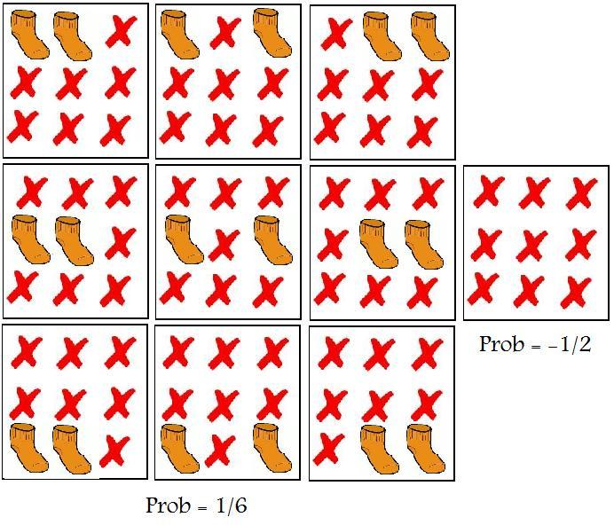
Ok, here is a probabilistic description of Albert's drawers. A total of 10 configurations are relevant:

1. Nine configurations consist of two drawers in a single row being filled, and all other drawers being empty. These nine configurations each carry a 1/6 probability.
2. One additional configuration features an empty chest of drawers. This configuration carries a minus 1/2 probability.

It is easy to see that all probabilities add up to unity, as they should. The negative probability for the 'all empty' state is a strange beast, but a beast that doesn't show up in the end result when calculating observable probabilities.

For instance, let's calculate the probabilities for observing the various numbers of socks in the bottom row of Albert's chest. In the above table you can read off that we have seven realizations with an empty bottom row, six with +1/6 probability, and one with –1/2 probability. The total probability for an empty bottom row is therefore +1/2. Furthermore, we have three realizations with a bottom row filled with two socks, each with a probability of +1/6. The total probability for finding two socks in the bottom row is therefore +1/2. So we have two equal likelihoods of finding zero or two socks, each with a positive (+1/2) value, and we are guaranteed to retrieve an even number of socks from the bottom row.

Repeating the same calculation for a column leads to the result that a column renders one sock with unit probability, hence a guarantee for an outcome of an odd number of socks.

What happened in both these cases is that the negative probability gets cancelled by positive probabilities describing the same outcome for the row or column under consideration. As a result, rows lead to even numbers and columns to odd numbers, and never does a negative probability turn up its ugly head.

This obviously doesn't hold when determining the number of socks in the entire chest of drawers. A negative probability does show up prominently, and it does not get cancelled as there are no positive probabilities describing the same configuration. However, we don't need to worry about this, as the configuration with negative probability does not correspond to a possible observation. Only three drawers (one row or one column) can be opened, not the whole chest.

What this means is that one can extract only a limited amount of information out of Albert's chest. Getting more information out of it (opening more drawers) is impossible as it would lead to negative probabilities to become evident. This is a manifestation of Heisenberg's uncertainty principle for Albert's chest.

Heisenberg uncertainty, destructive interference, spooky action at a distance, violation of Bell's inequalities, all of quantum physics can be mapped on negative probability models. So why don't physicists use such negative probability models? The answer is simple: negative probability models are rather clumsy representations of what is better described using "Pythagorean probabilities".

But as a model to get some understanding of the fundamentals of quantum physics, negative probability models do carry a value largely unexplored by pop-science writers.

All of this places some of Einstein's quotes in a different light.

God does play dice. And malicious he is. Or how would you characterize anyone who throws dice loaded to render negative chances, and who manages to keep this so well-hidden from us?

---

Disclaimer by LM: The views and opinions expressed in this article are those of the author but they do reflect the position of TRF. By the way, if you want the relevant operators etc., the closest discussion on TRF is this treatment of the GHZM experiment. For those who want the realization of this particular "drawer", it's caller the Mermin-Peres magic square (thanks, Johannes) and it acts on just two qubits (two spins). The \(3\times 3\) operators are\[

\begin{array}{|c|c|c|}
\hline
\,1\otimes \sigma_z& \sigma_z\otimes 1& \sigma_z\otimes\sigma_z\\
\hline
\sigma_x\otimes 1\,& \,1\otimes \sigma_x& \sigma_x\otimes \sigma_x\\
\hline
-\sigma_x\otimes \sigma_z&- \sigma_z\otimes \sigma_x &\sigma_y\otimes \sigma_y\\
\hline
\end{array}

\] Each pair of operators in the same row commutes; each pair in the same column commutes. Check it. The third entry in each row is a product of the previous two so the "even number of socks in each row" is guaranteed. I added minus signs on the third row so that the product in each column is \(-1\), too. Note that for the individual drawer measurements, \((+1)=\)"yes sock" and \((-1)=\)"no sock". So the correlations are guaranteed regardless of the state vector.

It's left as an exercise to the reader to determine the state vector for which the probabilities are as indicated by Johannes; and to find out how the Wigner distribution which has 9 times +1/6 and 1 times –1/2 should be constructed.

This magic square has been used as a tool in quantum pseudo-telepathy and exaggerations of this sexy term are guaranteed. ;-)

Different ways to interpret Feynman diagrams

Feynman diagrams are the funny pictures that Richard Feynman drew on his van:



You see that a Feynman diagram is composed of several lines that meet at vertices (at the nodes of the graph). Some of the lines are straight, some of them are wiggly: this shape of each line distinguishes the particle type. For example, straight lines are often reserved for fermions while wiggly lines are reserved for photons or other gauge bosons.




Some lines (I mean line intervals) are external – one of their two endpoints is free, unattached to anything. These are the external physical particles that must obey the mass on-shell condition \(p_\mu p^\mu = m^2\) and that specify the problem we're solving (i.e. what's the probability that some particular collection of particles with some momenta and polarization will scatter and produce another or the same collection particles with other momenta and polarizations). Other lines (I mean line intervals) are internal and they are unconstrained. You must sum over all possible ways to connect the predetermined external lines by allowed vertices and allowed internal lines. If you associate a momentum with these internal lines, also known as "propagators", it doesn't have to obey the mass on-shell condition. We say that the particle is "virtual". An explanation why its \(E\) may differ from \(\sqrt{p^2+m^2}\) is that the virtual particle only exists temporarily and the energy can't be accurately measured or imposed because of the inequality \(\Delta E\cdot\Delta t\geq\hbar/2\).

Because the virtual particles are not external, they define neither the initial state nor the final state. Still, they "temporarily appear" during the process, e.g. scattering, and they influence what's happening. In fact, they're needed for almost every interaction. Also, the Feynman diagrams have vertices at which several lines meet, where they terminate. The vertices describe the real events in the spacetime in which the particles merge, splht, or otherwise interact. However, we're doing quantum mechanics so none of these points in spacetime are uniquely or objectively determined. In fact, all the choices contribute to the calculable results – the total probability amplitudes.

A Feynman diagram is a compact picture that may be drawn by most kids in the kindergarten. However, each Feynman diagram – assuming we know the context and conventions – may also be uniquely translated to an integral, a contribution to the complex "probability amplitude" whose total value is used to calculate the probability of any process in quantum field theory. The laws used to translate the kindergarten picture to a particular integral or a related mathematical expression are known as the "Feynman rules".

How do we derive them?

I will discuss three seemingly very different methods:

• Dyson's series, an operator-based method
• Feynman's sum over histories i.e. configurations of fields
• Feynman's sum over histories i.e. trajectories of first-quantized particles

Richard Feynman originally derived his Feynman diagrams by the second method. As his name in the description of a method indicates, Freeman Dyson rederived the Feynman rules for the Feynman diagrams using the first method – and it was an important moment from a marketing viewpoint because this is how Freeman Dyson made Feynman diagrams extremely popular and essentially omnipresent.

The third method was added for the sake of conceptual completeness and it is the least rigorous one. However, it still gives you another way to think about the origin of Feynman diagrams – a way that is perhaps generalized in the "most straightforward way" if you try to construct Feynman diagrams for perturbative string theory.

It's important to mention that Feynman has discovered many things and methods, of course, but we shouldn't confuse them. The Feynman diagrams are the pictures on the van, tools to calculate scattering amplitudes and Green's functions. But he also invented the Feynman path integral ("sum over histories") approach to any quantum mechanical theory. It's not quite the same thing as the Feynman diagrams – it applies to any quantum theory, not just quantum field theory. However, as I have already said, he used the "sum over histories" of a quantum field theory to derive the Feynman diagrams for the first time.

Two other, conceptually differently looking ways to derive the Feynman diagrams were found later. The third method uses the "sum over histories" but applied to a "differently formulated system" than Feynman originally chose; the first method due to Dyson doesn't use the "sum over histories" at all.

Quadratic terms in the action, higher-order terms in the action

But all the three strategies to derive the Feynman rules share certain technical principles which are "independent of the formalism":

• The lines, both the propagators and the external lines, are associated with individual fields or particle species and with the bilinear or quadratic terms they contribute to the action (and the Lagrangian or the Hamiltonian).
• The vertices are associated with cubic, quartic, or other higher-order terms in the action (and the Lagrangian or the Hamiltonian), assuming that it is written in a polynomial form.

Let's assume we have an action and the Lagrangian that depends on the fields \(\phi_i\) in a polynomial way:\[

\eq{
\LL &= a_0 + \sum_i a_{1,i} \phi_i + \frac{1}{2!} \sum_{i,j} a_{2,ij} \phi_i\phi_j +\\
&+ \frac{1}{3!}\sum_{i,j,k} a_{3,ijk} \phi_i\phi_j\phi_k+\dots
}

\] which continues to higher orders, if needed, and which also contains various similar terms with the (first or higher-order) spacetime derivatives \(\partial_\mu\) of the fields \(\phi_i\) contracted in various ways. We don't consider the spacetime derivatives as something that affects the order in \(\phi\) so \(\partial_\mu \phi\partial^\mu \phi\) is still a second-order term in \(\phi\). The number of fields \(\phi_i\) – the order in \(\phi\) – that appear in the cubic or higher-order term will determine how many lines are attached to the corresponding vertex of the Feynman diagram.

The individual coefficients \(a_{n,i}\) etc. are parameters or "coupling constants" of a sort. How do we treat them?

Well, the first term, the universal constant \(a_0\), is some sort of the vacuum energy density. As long as we consider dynamics without gravity, it won't affect anything that may be observed. For example, the classical (or Heisenberg) equations of motion for the operators are unaffected because the derivative of a constant such as \(a_0\) with respect to any degree of freedom vanishes. We know that even in the Newtonian physics, the overall additive shift to energy is a matter of conventions. The potential energy is \(mgh\) where \(h\) is the height but you may interpret it as the weight above your table or above the sea level or above any other level and Newton's equations still work.

If we include gravity, the term \(a_0\) acts like a cosmological constant and it curves the spacetime. Fine. We will ignore gravity here so we will ignore \(a_0\), too.

The next terms are linear, proportional to \(a_{1,i}\). They are multiplied by one copy of a quantum field. For the Lorentz invariance to hold, it should better be a scalar field and if it is not, it must be a bosonic field and the vector indices must be contracted with those of some derivatives, e.g. as in \(\partial_\mu A^\mu\).

What do we do with the linear terms?

Well, here we can't say that they don't matter. They do depend on the fields and they do matter. But we will still erase them because of a different reason: they matter too much. If the potential energy contains a term proportional to \(\phi\) near \(\phi=0\), it means that \(\phi=0\) isn't a stationary point. The value of \(\phi\) will try to "roll down" in one of the directions to minimize the potential energy. It will either do so indefinitely, in which case the Universe is a catastrophically unstable hell, or it will ultimately reach a local minimum of the potential energy. In the latter, peaceful case, you may expand around \(\phi=\phi_{\rm min}\), i.e. around the new minimum, and if you do so, the linear terms will be absent.

So if we perform these basic steps, we see that without a loss of generality, we may assume that the Lagrangian only begins with the bilinear or quadratic terms. The following ones are cubic, and so on.

(We could start with a quantum field theory that has nontrivial linear terms, e.g. in the scalar field, anyway. In that case, the instability of the "vacuum" we assumed would manifest itself by a non-vanishing "one-point functions" for the relevant scalar field(s). The Feynman diagrams for these one-point functions ("scattering of a 1-particle state to a 0-particle state or vice versa") are known as "tadpoles" – tadpoles have a loop(s)/head and one external leg – because a journal editor decided that Sidney Coleman's alternative term for these diagrams, the "spermion", was even more problematic than a "tadpole".)

Bilinear terms and propagators

The method of Feynman diagrams typically assumes that we are expanding around a "free field theory". A free field theory is one that isn't interacting. What does it mathematically mean? It means that its Lagrangian is purely bilinear or quadratic. If we want to extract the "relevant" bilinear Lagrangian out of a theory that has many higher-order terms as well, we simply erase the higher-order terms.

Why is a quadratic Lagrangian defining a "free theory"? It's because by taking the variation, it implies equations of motions for the fields that are linear. And linear equations obey the superposition principle: if \(\phi_A(\vec x,t)\) and \(\phi_B(\vec x,t)\) are solutions to the equations of motion, so is \(\phi_A+\phi_B\). If \(\phi_A\) describes a wave packet moving in one direction and \(\phi_B\) describes a wave packet moving in another direction, they may intersect or overlap but the wave packets may be simply added which means that they pretend that they don't see one another: they just penetrate through their friend. This is the reason why they don't interact. Linear equations describe waves that just freely propagate and don't care about anyone else. Linear equations are derived from quadratic or bilinear actions. That's why quadratic or bilinear actions define "free field theories".

If we appropriately integrate by parts, we may bring the bilinear terms to the form\[

\LL_{\rm free}=\frac{1}{2}\sum_{ij} C_{ij} \phi_i P_{ij} \phi_j

\] where \(P_{ij}\) is some operator, for example \((\partial_\mu\partial^\mu+m^2)\delta_{ij}\). The factor \(1/2\) is a convention that is natural because if we differentiate the expression above with respect to a \(\phi_i\), we produce two identical terms due to the Leibniz rule for the derivative of the product. (That's not the case if the first \(\phi_i\) were \(\phi^*_i\) which is needed when it's complex: for complex fields, including the Dirac fields etc., the factor of \(1/2\) is naturally dropped.)

So the classical equations of motion derived for those fields look like this:\[

\sum_j P_{ij} \phi_j = 0.

\] You should imagine the Klein-Gordon equation as an example of such an equation.

Some operator, e.g. the box operator, acts on the fields and gives you zero. These are linear equations. You may often explicitly write down solutions such as plane waves, \(\phi_i = \exp(ip\cdot x)\), and all their linear superpositions are solutions as well. The coefficients of these plane waves are called creation and annihilation operators etc. You may derive what spectrum of free particles may be produced by a free field theory.

This may be done in the operator approach – the free fields are infinite-dimensional harmonic oscillators defined by their raising and lowering operators – as well as by the "sum over histories" approach – the harmonic oscillator may be solved in this way as well. The "sum over histories" approach encourages you to choose the \(\ket x\) or \(\ket{ \{\phi_i(\vec x,t)\} }\) continuous (or functionally metacontinuous) basis of the Hilbert space. By the functionally metacontinuous basis, I mean a basis that gives you a basis vector for each function or \(n\)-tuple of functions \( \{\phi_i(\vec x,t=t_0) \} \) even though these functions form a set that is not only continuous but actually infinite-dimensional.

But I want to focus on the derivation of the Feynman rules including the vertices. We don't want to spend hours with a free field theory. When we construct the Feynman rules, the free part of the action determines the particles that may be created and annihilated and that define the initial and final Hilbert space as a Fock space; and it determines the propagators.

The propagators will be determined by "simply" inverting the operator \(P_{ij}\) I used to define the bilinear action above. This inverted \(P^{-1}_{ij}\) plays the role of the propagator for a simple reason: we ultimately need to solve the linear equation of motion with some function on the right hand side. Each function may be written as a combination of continuously infinitely many (i.e. as an integral over) delta-functions so we really need to solve the equation\[

\sum_j P_{ij} \phi_j = \delta^{(4)} (x-x') \cdot k_i

\] for some coefficients \(k_i\) – which may be decomposed into Kronecker deltas \(\delta_{im}\) for individual values of \(m\). The value of \(x'\) – the spacetime event where the delta-function is localized – doesn't change anything profound about the equation due to the translational symmetry. A funny thing is that the equation above may be formally solved by multiplying it with the inverse operator:\[

\phi_i = \sum_j P^{-1}_{ij} \delta^{(4)}(x-x')\cdot k_j.

\] That's why the inverse of the operator \(P_{ij}\) – which is nonlocal (the opposite to differentiation is integration and we are generalizing this fact) appears in the Feynman rules.

So far I am presenting features of the results "informally"; we are not strictly deriving any Feynman rules and we haven't chosen one of the three methods yet.

Higher-order terms

I will postpone this point but the cubic and higher-order terms in the Lagrangian will produce the vertices of the Feynman diagrams. In the position representation, the locations of the vertices must be integrated over the whole spacetime.

In the momentum representation, the vertices are interactions that appear "everywhere" and we must instead impose the 4-momentum conservation at each vertex. In the latter approach, some momenta will continue to be undetermined even if the external particles' momenta are given. The more independent "loops" the Feynman diagram has, the more independent momenta running through the propagators must be specified. All the allowed values of the loop momenta must be integrated over.

The momentum and position approaches are related by the Fourier transform. Note that the Fourier transform of a product is a "convolution" and this is the sort of mathematical facts that translates the rules from the momentum representation to the position representation and vice versa.

Starting with the methods: Dyson series

We have already leaked what the final Feynman rules should look like so let us try to derive them. Dyson's method coincides with the tools in quantum mechanics that most courses teach you at the beginning, so it's a beginner-friendly method (although this statement depends on our culture and on those perhaps suboptimal ways how we teach quantum mechanics and quantum field theory). But it's actually not the first method by which the Feynman rules were derived; Feynman originally used the "sum over histories" applied to fields.

Dyson's method uses several useful technicalities, namely the Dirac interaction picture; time ordering; and a modified Taylor expansion for the exponential.

The Dirac interaction picture is a clever compromise between Schrödinger's picture in which the operators are independent of time and the state vector evolves according to Schrödinger's equation that depends on the Hamiltonian; and the Heisenberg picture in which the state vector is independent of time and the operators evolve according the Heisenberg equations of motion that resemble the classical equations of motion with extra hats (which are omitted on this blog because it's a quantum mechanical blog).

In the Dirac interaction picture, we divide the Hamiltonian to the "easy", bilinear part we have discussed above and this "free part" is used for the Heisenberg-like evolution equations (the operators evolve in a simple linear way as a result); and the "hard", higher-order or interacting part of the Hamiltonian which is used as "the" Hamiltonian in a Schrödinger-like equation. So we have:\[

\eq{
H(t) &= H_0 + V(t), \\
i\hbar \pfrac{\phi_i(\vec x,t)}{t} &= [\phi_i(\vec x,t),H_0]\\
i\hbar \ddfrac{\ket{\psi(t)}}{t} &= V(t)\ket{\psi(t)}.
}

\] The operators evolve according to \(H_0\), the free part, but the wave function evolves according to \(V(t)\). Note that \(V(t)\) – and of course the whole \(H(t)\) as well – is a rather general composite operator so it also depends on time: its evolution is also determined by its commutator with \(H_0\). On the other hand, \(H_0\) itself, while an operator, is \(t\)-independent because it commutes with itself.

The operator \(H_0\) depends on the elementary fields \(\phi_i\) in a quadratic way so the commutator in the second, Heisenberg-like equation above is linear in the fields \(\phi_i\). Consequently, these equations of motion are "solvable" and the solutions may be written as some combinations of the plane waves – the usual decomposition of operators \(\phi_i(\vec x,t)\) into plane waves multiplied by coefficients that are interpreted as creation and annihilation operators.

The proof that this Dirac interaction picture is equivalent to either Heisenberg or Schrödinger picture is analogous to the proof of the equivalence of the latter two pictures themselves; one just considers "something in between them".

Getting the time-ordered exponential

At any rate, we may now ask how the initial state \(\ket\psi\) at \(t=-\infty\) evolves to the final state at \(t=+\infty\) via the Schrödinger-like equation that only contains the interacting (higher-order) \(V(t)\) part of the Hamiltonian. We may divide the evolution into infinitely many infinitesimal steps by \(\epsilon\equiv \Delta t\). The evolution in each step (the process of waiting for time \(\epsilon\)) is given by the map\[

\ket\psi \mapsto \zav{ 1+\frac{\epsilon}{i\hbar} V(t) }\ket\psi.

\] For an infinitesimal \(\epsilon\), the terms that are higher-order in \(\epsilon\) may be neglected. To exploit the formula above, we must simply perform this map infinitely many times on the initial \(\ket\psi\). Imagine that one day is very short and its length is \(\epsilon\) and use the symbol \(U_t\) for the parenthesis \(1+\epsilon V(t)/i\hbar \) above. Then the evolution over the first six days of the week will be given by\[

\ket\psi \mapsto U_{\rm Sat} U_{\rm Fri} U_{\rm Thu} U_{\rm Wed} U_{\rm Tue} U_{\rm Mon}\ket\psi.

\] Note that the Monday evolution operator acts first on the ket, so it appears on the right end of the product of evolution operators. The later day we consider, the further on the left side – further from the ket vector – it appears in the product. So the evolution from Monday to Saturday (or Sunday) is given by a product where the later operators are always placed on the left side from the earlier ones. We call such products of operators "time-ordered products".

In fact, we may define a "metaoperator" of time-ordering \({\mathcal T}\) which, if it acts on things like \(V(\text{Day1}) V(\text{Day2})\), produces the product of the operators in the right order, with the later ones standing on the left. The ordering is important because operators usually refuse to commute with each other in quantum mechanics.

Now, if you study the product of the \(U_{\rm Day}\) operators above, you will realize that the product generalizes our favorite "moderate interest rates still yield the exponential growth at the end" formula for the exponential\[

\exp(X) = \lim_{N\to \infty} \zav{ 1 + \frac XN }^N

\] where \(1/N\) may be identified with \(\epsilon\). The generalization affects two features of this formula. First, the terms \(X/N\) aren't constant, i.e. independent of \(t\), but they gradually evolve with \(t\) because they depend on \(V(t)\). Second, we mustn't forget about the time ordering. Both modifications are easily incorporated. The first one is acknowledged by writing \(X\) inside \(\exp(X)\) as the integral over time; the second one is taken into account by including the "metaoperator" of time-ordering. (I call it a "metaoperator" so that it suppresses your tendency to think that it's just an operator on the Hilbert space. It's not. It's an abstract symbol that does something with genuine operators on the Hilbert space. What it does is still linear – in the operators.)

With these modifications, we see that the evolution map is simply\[

\ket\psi\mapsto {\mathcal T} \exp\zav{ \int_{-\infty}^{+\infty}\dd t\, \zav{ \frac{V(t)}{i\hbar} } } \ket\psi

\] The time-ordered exponential is an explicit form for the evolution operator (the \(S\)-matrix) that simply evolves your Universe from minus infinity to plus infinity. In classical physics, you could rarely write such an evolution map explicitly but quantum mechanics is, in a certain sense, simpler. Linearity made it possible to "solve" the most general system by an explicit formula.

Once we have this "time-ordered exponential", we may deal with it in additional clever ways. The exponential may be Taylor-expanded, assuming that we don't forget about the time-ordering symbol in front of all the monomial terms in the Taylor expansion. The operators \(V(t)\) are polynomial in the fields and their spacetime derivatives: we allow each "elementary field" factor to either create or annihilate particles in the initial or final state (these elementary fields will become the inner end points of external lines of Feynman diagrams); or we keep the elementary fields "ready to perform internal services". In the latter case, we will need to know the correlators such as\[

\bra 0 \phi_i(\vec x,t) \phi_j(\vec x', t')\ket 0

\] which is a sort of a "response function" that may be calculated – even by the operator approaches – and which will play the role of the propagators. The remaining coefficients and tensor structures seen in \(V(t)\) will be imprinted to the Feynman rules for the vertices, the places where at least 3 lines meet.

I suppose you know these things or you will spend enough time with the derivation so that you understand many subtleties. My goal here isn't to go through one particular method in detail, however. My goal is to show you different ways how to look at the derivation of the Feynman diagrams. They seem conceptually or philosophically very different although the final predictions for the probability amplitudes are exactly equivalent.

Feynman's original method: "sum over histories" of fields

Feynman originally derived the Feynman rules by "summing over histories" of fields. The very point of the "sum over histories" approach to quantum mechanics is that we consider a classical system, the classical limit of the quantum system we want to describe, and consider all of its histories, including (and especially) those that violate the classical equations of motion. For each such a history or configuration in the spacetime, we calculate the action \(S\), and we sum i.e. integrate \(\exp(iS/\hbar)\) over all these histories, perhaps with the extra condition that the initial and final configurations agree with the specified ones (those that define the problem we want to calculate).

(See Feynman's thesis: arrival of path integrals, Why path integrals agree with the uncertainty principle, and other texts about path integrals.)

We have already mentioned that we're dividing the action, Lagrangian, or Hamiltonian to the "free part" and the "interacting part". We're doing the same thing if we use this Feynman's original method, too. To deal with the external lines, we have to describe the wave functions (or wave functionals) for the multiparticle states; this task generalizes the analogous problem with the quantum harmonic oscillator to the case of the infinite dimension and I won't discuss it in detail.

What's more important are the propagators, i.e. the internal lines, and the vertices. The propagators produce the inverse operator \(P_{ij}^{-1}\) from the Lagrangian again. These "Green's functions" have the property I have informally mentioned – they solve the "wave equation" with the Dirac delta-function on the right hand side; and they are equal to the two-point correlation functions evaluated in the vacuum.

But Feynman's path integral has a new way to derive the appearance of this inverse operator as the propagator. It boils down to the Gaussian integral\[

\int \dd^n x\,\exp(\vec x\cdot M\cdot \vec x) = \frac{\pi^{n/2}}{\sqrt{\det M}}.

\] but what is even more relevant is a modified version of this integral that has an extra linear term in the exponent aside from the bilinear piece:\[

\int \dd^n x\,\exp(\vec x\cdot M\cdot \vec x+ \vec J\cdot \vec x) = \dots

\] This more complicated integral may be solved by "completing the square" i.e. by the substitution\[

\vec x = \vec x' - \frac{1}{2} M^{-1}\cdot \vec J.

\] With this substitution, after we expand everything, the \(\vec x'\cdot \vec J\) "mixed terms" get canceled. As a replacement, we produce an extra term\[

-\frac{1}{4} \vec J\cdot M^{-1} \cdot \vec J

\] in the exponent; the coefficient \(-1/4\) arises as \(+1/4-1/2\). And because \(M\) is the matrix that is generalized by our operator \(P_{ij}\) discussed previously, we see how the inverse \(P^{-1}_{ij}\) appears sandwiched in between two vectors \(\vec J\).

The strategy to evaluate the Feynman's path integral is to imagine that this whole integral is a "perturbation" of a Gaussian integral we know how to calculate. We work with all the \(V(\vec x,t)\) interaction terms as if they were general perturbations similar to the \(\vec J\) vector above, and in this way, we reproduce all the vertices and all the propagators again.

Note that I have been even more sketchy here because this text mainly serves as a remainder that there exists a "philosophically different attitude" to the Feynman diagrams that one shouldn't overlook or dismiss just because he got used to other techniques and a different philosophy. If you want to calculate things, it's good to learn one method and ignore most of the others so that you're not distracted. But once you start to think about philosophy and generalizations, you shouldn't allow your – often random and idiosyncratic – habits to make you narrow-minded and to encourage you to overlook that there are completely different ways how to think about the same physics. These different ways to think about physics often lead to different kinds of "straightforward generalizations" that might look very unnatural or "difficult to invent" in other approaches.

In science, one must disentangle insights that are established – directly or indirectly supported by the experimental data – from arbitrary philosophical fads that you may be promoting just because you got used to them or for other not-quite-serious reasons. Of course, this broader point is the actual important punch line I am trying to convey by looking at a particular technical problem, namely methods to derive the Feynman rules.

Feynman's other method: "sum over histories" of merging and splitting particles

Once I have unmasked my real agenda, I will be even more sketchy when it comes to the third philosophical paradigm. You may "derive" the Feynman rules, at least qualitatively, from the "first-quantized approach" emulating non-relativistic quantum mechanics.

Again, in this derivation, we are "summing over histories". But they're not "histories of the fields \(\phi_i(\vec x,t)\)" as in the approach from the previous section – the original method Feynman exploited to derive the Feynman rules. Instead, we may sum over histories of ordinary mechanics, i.e. over histories of trajectories \(\vec x(t)\) for different particles in the process.

This approach, emulating non-relativistic quantum mechanics, the propagators \(D(x,y)\) arise as the probability amplitude for a particle to get from the point \(x\) of the spacetime to the point \(y\). It just happens that the form of the propagators – which have been interpreted as matrix elements of the "inverse wave operator" \(P^{-1}_{ij}\); and as two-points functions evaluated in the vacuum – may also be interpreted as the amplitude for a particle getting from one point to another.

Well, this works in some approximations and one needs to deal with antiparticles properly in order to restore the Lorentz invariance and causality (note that the sum over particles' trajectories still deals with trajectories that are superluminal almost everywhere, but the final result still obeys the restrictions and symmetries of relativity!) and it's tough. At the end, the "derivation" ends up being a heuristic one.

But morally speaking, it works. In this interpretation, a Feynman diagram encodes some histories of point-like particles that propagate in the spacetime and that merge or split at the vertices which correspond to spacetime points at which the total number of particles in the Universe may change (this step would be unusual in non-relativistic quantum mechanics, of course). The path integral over all the paths of the internal particles gives us the propagators; the vertices where the particles split or join must be accompanied by the right prefactors, index contractions, and other algebraic structures. But in some sense, it works.

It's this interpretation of the Feynman diagrams that has the most straightforward generalization in string theory. In string theory, we may imagine cylindrical or strip-like world sheets – histories of a single closed string or a single open string propagating in time – and they generalize the world lines. The path integral over all histories like that, between the initial closed/open string state and the final one, gives us a generalized Green's function for a single string.

And in string theory, we simply allow the topology of the world sheet to bd nontrivial – to resemble the pants diagram or the genus \(h\) surface with additional boundaries or crosscaps – and it's enough (as well as the only consistent way) to introduce interactions. While the interactions of point-like particles are given by vertices, "singular places" of the Feynman diagrams, and this singular character of the vertices is ultimately responsible for all the short-distance problems in quantum field theories, the world sheets for strings have no singular places at all. They're smooth manifolds – each open set is diffeomorphic to a subset of \(\RR^2\), especially if you work in the Euclidean signature – but if you look at a manifold globally (and only if you do so), you may determine its topology and say whether some interactions have taken place.

So this third method of interpreting the Feynman diagrams – as the sum over histories of point-like particles in the spacetime that are allowed to split and join at the vertices – which was the "most heuristic one" and the "method that was least connected to exact formulae" encoding the mathematical expressions behind the Feynman diagrams actually becomes the most straightforward, the most rigorous way to derive the analogous amplitudes in string theory.



Take the world from another point of view, interview with RPF, 36 minutes, PBS NOVA 1973. At 0:40, he also mentions that brushing your teeth is a superstition. Given my recent appreciation of the yeasts that are unaffected by the regular toothpastes, I started to think RPF had a point about this issue, too.

If you got stuck with a particular "philosophy" how to derive the Feynman rules, e.g. with Dyson's series, it could be much harder – but not impossible – to derive the mathematical expressions for multiloop string diagrams. There have been many methods due to Richard Feynman mentioned in this text but once again, the most far-reaching philosophical lesson is one that may be attributed to Richard Feynman as well:

Perhaps Feynman's most unique and towering ability was his compulsive need to do things from scratch, work out everything from first principles, understand it inside out, backwards and forwards and from as many different angles as possible.

I took the sentence from a review of a book about Feynman. It's great if you decompose things to the smallest possible blocks, rediscover them from scratch, and try to look at the pieces out of which the theoretical structure is composed from as many angles as you can. New perspectives may give you new insights, new perceptions of a deeper understanding, and new opportunities to find new laws and generalize them in ways that others couldn't think of.

And that's the memo.

P.S.: BBC and Discovery's Science Channel plan to shoot a Feynman-centered historical drama about the Challenger tragedy.



Prayer for Marta ["Let the peace remain with this land. Let anger, envy, jealousy, fear and conflicts subside, let them subside. Now when your lost control over your things will return to you, the people, it will return to you..."], an iconic politically flavored 1968 song by which the singer restarted freedom lost in 1968 during the Velvet Revolution in 1989.

P.P.S.: Ms Marta Kubišová, a top Czech pop singer in the late 1960s (Youtube videos), refused to co-operate with the pro-occupation establishment after the 1968 Soviet invasion which is why she became a harassed clerk in a vegetable shop rather than a pillar of the totalitarian entertainment similar to her ex-friend Ms Helena Vondráčková.

She just received Napoleon Bonaparte's Legion of Honor award, a well deserved one. Congratulations!